.Figure 2

.
.
.
.
.
.
.
.
Figure 3
Current Account Transactions:
1. Merchandise Balance = Exports - Imports of Goods
2. Net Exports (Trade Balance, NX) = Merchandise Balance plus Net Exports of Services Figure 1
3. Current Account Balance (CA) = Trade Balance + Net Factor Income from Abroad ( = NX + i NFA).
A country running a CA deficit must finance this deficit
through net borrowing from the rest of the world (i.e. either by by increasing
its net debt or by reducing its net foreign assets).
If NFA is the net stock of foreign assets held by people in the United States (US ownership of foreign assets, net of foreign ownership of US assets), then changes in NFA are equal to the current account:
NFAt+1 = NFAt + CAt .
NFAt+1= NFAt + GDPt + it NFAt - Ct - Gt - It = NFAt + CAt
Another way of seeing the relation between the CA and the NFA of the country: link between the current account of the BP (that records current transactions, i.e. trade in goods and services and the interest payments on net foreign assets) and the capital account of the BP (that records capital transactions, i.e. the purchase and sale of foreign assets).
The sum of the current account (CA) and capital account (KA) of the balance of payments is equal to the change in the official foreign reserves of the country (d(FAX) or:
CA + KA = d(FAX) (1)
Suppose that the change in official foreign reserves is zero (d(FAX)=0); then:
CA+KA=0
If you have a current account deficit, say CA = -50 < 0), you need a capital inflow (net new borrowing) from the rest of the world to finance this CA imbalance. Since you are borrowing from the rest of the world, the increase in our foreign debt is a capital inflow (as foreign residents are buying domestic securities, bonds, equities, or extend bank credit/loans to domestic agents). Therefore, a current account deficit (CA= -50 <0) is associated by a matching and equivalent positive capital inflow (KA = 50 >0) that is represented by a positive item in the Capital Account of the balance of payments (KA = 50 >0). Since the capital inflow is equal to the negative of the CA deficit (KA = 50= - CA = -(-50)), we get that CA+KA =0.
Now introduce official foreign reserves (of the central bank). If the country is running a $50b current account deficit, that needs to be financed with an equivalent net capital inflow. Suppose, however, that foreign agents are willing to lend only $30b to the domestic economy, i.e. the positive capital inflow (KA) is only $30b. Then, the only way that the country can finance its current account deficit is to run down its official foreign assets (i.e. the reserves of the central banks). In other terms, if foreign agents are not willing to lend funds to domestic agents to finance the CA deficit, the domestic agents will go to the central bank, purchase foreign currency from the central banks that they pay for buy paying with domestic currency (money); then, they will use this foreign currency to pay for the excess of imports over exports. This set of transactions will lead to a reduction in the stock of official foreign assets (foreign reserves) of the central bank. The change in the stock of official foreign reserves (d(FAX)) will therefore be equal to excess of the current account deficit relative to the capital inflow or:
d(FAX) = CA + KA
-20 = -50 + 30
Formally, the capital account is:
KAt = Capital inflows - Capital outflows = Change in foreign liabilities - change in private sector foreign assets
Example: Korea in 1996 (all data in billions of US dollars):
Equivalent line in IMF
International Financial
Statistics
Trade Balance on Goods -15.3 78acd
Trade Balance on Services -5.3 78add - 78aed
Overall Balance on Goods and Services -20.6 78afd
Net Foreign Income From Abroad:
-2.5
78agd-78ahd
of which:
Income paid
-5.3
78ahd
Income received
+2.8
78agd
Balance on Goods, Services and Income -23.1 78aid
Net (Unilateral) Current Transfers
0.1
78ajd - 78akd
of which:
Transfers made
-4.3
78akd
Transfers received
+4.4
78ajd
Current Account (CA):
-23.0
78ald = 78afd +(78ajd-78akd)
.
Capital Account (KA):
+24.4 = 43.6 - 19.2 (Cap. Inflows - Cap. Outflows)
.
.
Capital Inflows:
43.6
of which:
Foreign Portfolio investments in Korea
16.7
78bgd
(foreign purchases of Korean stocks and bonds)
Other investments
23.6
78bid
(mostly foreign lending to Korean banks)
Foreign Direct Investment into Korea 2.3 78bed
Unreported Capital Inflows
1.0
78cad
(Errors and Omissions line of BP accounts)
Other Capital Account Items
0.0
78bad
Capital Outflows: -19.2
of which:
Portfolio investments by Korean abroad
-2.4
78bfd
(Korean purchases of foreign stocks and bonds)
Other investments
-11.8
78bhd
(mostly lending by Korean banks to foreign agents)
FDI by Korean firms in other countries -4.4 78bdd
Other Capital Account Items
-0.6
78bbd
Change in the Official Foreign Reserves
1.4 = -23.0 + 24.4
78cbd
(of the Korean Central Bank) d(FAX)
1. Stock of Foreign Reserves. The existence of large foreign exchange reserves will facilitate the financing of the current account deficit especially when the country is pegging its exchange rate and needs foreign reserves to credibly fix its exchange rate. Foreign exchange reserves reduce the risk of unsustainability and enable a country to finance a current account deficit at lower cost.
2. The composition and size of the capital inflows. The composition of the capital inflows necessary to finance a given current account deficit is an important determinant of sustainability. Short-term capital inflows are more dangerous than long-term flows and equity inflows are more stable than debt-creating inflows. A current account deficit that is financed by large foreign direct investment (FDI) is more sustainable than a deficit financed by short-term "hot money" flows. Among the debt-creating inflows, those from official creditors are more stable and less reversible in the short-run than those coming from private creditors; those taking the form of loans from foreign banks are usually less volatile than portfolio inflows (bonds and non-FDI equity investments). Asia caveat.
3. The stock of foreign debt burden. The current account deficit needs to be financed by a capital inflow or accumulation of debt. The ability to sustain deficits will be affected by the countrys stock of international assets. An existing large burden of international debt will make it more difficult to finance a current account imbalance. Things are particularly fragile when, as in Mexico in 1994 and in Asia in 1997, a large fraction of the foreign debt consists of short-term liabilities that have to be rolled-over in the short-run. If currency crisis leads to a panic in the financial markets, international creditors may be unwilling to roll-over these loans and the currency crisis can turn into a debt crisis where the country risks to default on its foreign debt liabilities.
4. Fragility of the financial system. The soundness of the domestic financial system, particularly the banks, has bearing on a countrys ability to sustain a current account deficit. Capital inflows require a large intermediation role of domestic banks. However domestic banking crises are common in developing and emerging economies. They are the direct result of bad lending practices, often due to political influences on bank lending or the requirement that banks (which are often state owned) allocate credit to sustain state owned enterprises.
5. Political instability and uncertainty about the economic environment. Political instability or mere uncertainty about the course of economic policy will have much the same consequences as banking sector instability. The threat of a change in regime or of a regime that is not committed to sound macroeconomics policies can reduce the willingness of the international financial community to provide financing for a current account deficit.
Nominal and Real Exchange Rates and the PPP
Exchange rates. We use the convention that prices of foreign currency are expressed in dollars. This leads to the confusing result that increases in the exchange rate are decreases in the value of the dollar. Note: the financial sector convention is to define the exchange rate of the US $ as units of foreign currency per units domestic currency (daily data shown here), i.e. Yen per US dollars, that is the opposite of the convention we follow here ($ per Yen). (If confused, use an on-line Currency Convertor).
Our Definition:
The Exchange Rate is the Dollar Price of Foreign Currency
S$/YEN = Dollars needed to buy one Yen (say 0.86 US cents or 0.0086 Dollars)
S$/E = Dollars needed to buy one Euro (say $ 0.95)
If S increases the Dollar is Depreciating (it takes more $ to buy one unit of foreign currency).
If S decreases the Dollar is Appreciating (it takes less $ to buy one unit of foreign currency).
Alternative Definition (used in financial markets):
The Exchange Rate is the Foreign Currency Price of a US $
SYEN/$ = Yen needed to buy one US$ (say 116 Yen=1/0.008). See Figure2
SE/$ = Euros needed to buy one US $ (say 1.052 Euros = 1/0.95). See $/E
Exchange rates are very variable (see the Minneapolis Fed home page for updated Charts of U.S. exchange rates relative to a basket of currencies). (YEN/$)
Exchange rates are related to prices of foreign and domestic goods. Example:
P = price in $ of a unit of a domestic good (one gallon of gas, say $1.20)
Pf = price in units of foreign currency of the same good in a foreign country (say Euro 1.4)
Which good is more expensive ? The price in dollars (P$f) of a unit of the foreign good is equal to its price in foreign currency (Pf = Euro 1.4) times the exchange rate of the dollar relative to the foreign currency (S = 0.95):
P$f = S Pf = 0.95 x 1.4 = 1.33
The relative price of the foreign good to the domestic good (defined as RER):
RER = S Pf / P = 1.33 / 1.20 = 1.108
where S is the (spot) exchange rate. The good in Europe is 10.8% more expensive (when expressed in same currency) than the same good in the U.S.
Often we use price indexes, like CPI or GDP deflators, representing baskets of goods. In this case the ratio RER is referred to as the real exchange rate. It indicates how expensive foreign goods are relative to domestic goods.
If domestic and foreign goods were very similar, and there were few barriers to trade, then when expressed in the same currency their price should be equal. In this case the RER would be equal to one and show no change.
In fact, if the price ratio differed from one, buyers in Europe would only buy in the cheap country (US), driving up prices there until foreign and domestic prices were equal. Thus prices of foreign and domestic goods, expressed in a common currency, should be the same, leading the RER to stay around one.
This theory, applied to the baskets of goods underlying aggregate price indexes, is referred to as purchasing power parity, (or PPP) since the purchasing power of a dollar is predicted to be the same in both countries:
P = S Pf (= P$f )
In the example above instead:
P =1.20 < S Pf =1.33 (divergence from PPP)
So how, can we reach a PPP equilibrium when the relative price differs from unity ? There are three alternative ways the equilibrium can be restored:
1. European prices could fall from E 1.4 to E 1.263 so that: P=1.20=SPf=0.95x1.263
2. US prices may go up from $1.20 to $ 1.33 so that: P=1.33=SPf=0.95x1.4
3. The $/Euro exchange rate could appreciate from 0.95 to 0.857 so that: P=1.20= S Pf = 0.857 x 1.4
In practice, all of the three effects will be at work in reality.
What is the evidence on the PPP ? If the PPP holds, the real exchange rate (RER) should be equal to one and constant over time. In fact,
RER = S Pf / P = P / P = 1 (if the PPP holds).
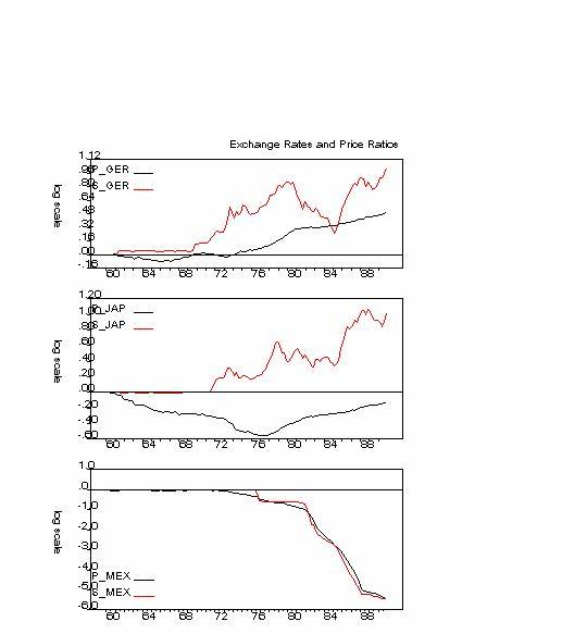
However, we find, when we compute RER using consumer price indexes, that it varies a lot: prices of (say) Mercedes in particular, and goods in general, are often much different in Germany/Europe and the US, and between any two other countries, as well. At least in the short-run, the PPP is a poor approximation.
Moreover, most of the variation in the RER is related to movements in the spot rate: see Figure 4 . In Figure 5 the real exchange rate is divided into two components: the ratio P/Pf is the solid line and the spot rate S is the dashed line. If PPP were true, the two lines would be the same (as PPP implies S = P/Pf). In fact they're much different.
Why the PPP does not hold in the short-run ? We assumed that the domestic and foreign goods were identical (a gallon of gasoline). However, the RER represents baskets of domestic and foreign goods that can be very different. Also, for homogenous goods, firms may price discriminate across markets.
While the PPP may not hold in the short-run, it should tend to hold in the long-run: if European prices are systematically higher than U.S. ones, at some point they will have to fall or US prices will have to go up, or the US $ will have to appreciate (or all of the above).
To understand the role of the exchange rate as an adjustment mechanism for relative prices and the trade balance, note the following points:
1. A depreciation (appreciation) of the domestic exchange rate makes foreign imported goods more expensive (cheaper) when priced in domestic currency. So a currency depreciation (appreciation) will lead to a reduction (increase) in the demand for imported goods as these goods become more expensive (cheaper). This reduction (increase) in the demand for imports should improve (worsen) the US trade balance.
2. A depreciation (appreciation) of the domestic exchange rate makes domestic goods exported abroad cheaper (more expensive) when priced in a foreign currency. So a currency depreciation (appreciation) will lead to a increase (decrease) in the foreign demand for US goods, i.e. an increase (decrease) in US exports as these goods become cheaper (more expensive) in foreign markets. This increase (decrease) in the US exports will improve (worsen) the US trade balance.
In particular:
1. A US$ appreciation decreases the price in US $ of imported goods (P$f) as: P$f =S Pf . So, a $ appreciation (an decrease in S) will decrease P$f . Example:
P$f = S Pf = 0.95 x 1.4 = 1.33
P$f = S Pf = 0.857 x 1.4 = 1.20
1. A US Dollar appreciation increases the price in foreign currency (Euro) of US goods exported abroad (PE ) since:
PE = P / S. So, a $ appreciation (an decrease in S) will increase PE. Example:
PE = P / S = 1.20 / 0.95 = 1.26
PDM = P / S = 1.20 / 0.857 = 1.4
So, a depreciation of the nominal exchange rate (S) will lead to an increase in the relative price of foreign to domestic goods, i.e. it will lead to a depreciation of the real exchange rate (RER). In fact:
RER = S Pf / P = P$f / P
If the price in own currency of domestic and foreign goods (P and Pf) is given, a nominal depreciaton of the exchange rate will also be a real depreciation.
Note: if the PPP was holding both in the short-run and the long-run, a nominal depreciation of the domestic currency would not lead to a depreciation of the real exchange rate. For given foreign prices of foreign goods, a nominal depreciation would increase proportionally by the same amount the price of imported goods and of domestic goods leaving the RER unaffected.
So, the PPP can be interpreted both as a theory of the determinant of the exchange rate and as a theory of the determinant of the domestic price level (or inflation rate). As theory of the exchange rate, the PPP can be written as:
S = P / Pf (1)
or, if we write the expression above in percentage rates of change:
dS/S = dP/P - dPf/Pf (2)
where dx/x is the percentage rate of change of variable x.
The expression (1) says that the exchange rate will be more depreciated if the domestic price level is higher than the foreign one (absolute PPP).
In rate of change form (relative PPP), expression (2) says that the exchange rate will depreciate at a % rate equal to the difference between domestic and foreign inflation. Example: if domestic inflation is 10% while foreign inflation is 4%, the domestic currency should depreciate on average by 6%.
The PPP, as a theory of the determinants of the exchange rate, considers the causality between P and S as going from domestic inflation to exchange rate depreciation: high inflation causes high depreciation rates.
As a theory of the determinants of the domestic inflation instead, the PPP considers the causality as going from the exchange rate to domestic inflation:
dP/P = dS/S + dPf/Pf (3)
(3) implies that, for given foreign inflation, the domestic inflation rate will be equal to the foreign inflation rate plus the 'exogenous' rate of depreciation of the domestic currency. For example, if foreign inflation is 4% and the domestic currency is depreciated by 20%, domestic inflation will be equal to 24%.
Of course, if the PPP does not strictly holds (at least in the short-run), the RER will not be always equal to one and constant and a depreciation of the nominal exchange rate will also depreciate the real exchange rate.
By how much will the real exchange rate depreciate if the nominal exchange rate depreciates by x% ?
0. Under PPP, the RER is unaffected as a currency depreciation increase the price of domestic goods by the same % rate as the currency depreciation.
1. If the domestic price level was completely independent of the nominal exchange rate, the domestic inflation rate would be totally unaffected by a nominal depreciation. In this case, the real exchange rate would depreciate by x% as well. This is an extreme case where the increase in the price of imported goods caused by the nominal depreciation does not affect at all the price of domestic goods.
2. If an x% nominal depreciation leads to an increase in domestic inflation (but by less than the x% implied by the PPP), the real exchange rate will depreciate but, by less than x%. In fact, by definition:
dRER/RER = dS/S + dPf/Pf - dP/P
Example: Mexico in 1995. Foreign (US) inflation was 3% while the Mexican Peso depreciated during the year by about 107%. If the Mexican inflation in 1995 has remained at the 1994 level (about 8%), the 107% nominal depreciation would have corresponded to a real depreciation of 102% (107 + 3 - 8). The large devaluation of 1995 led to an increase in the inflation rate that surged to 48% in 1995. So, the nominal depreciation of the Peso of 107% corresponded to a smaller real depreciation of 52% (107 + 3 - 48). Major improvement of the Mexican trade balance in 1995.
Implication. A currency devaluation is a double-sided sword:
1. On one side, it leads to a real depreciation that makes imported goods more expensive, domestic exports cheaper abroad and leads to an improvement of the trade balance via a fall in imports and an increase in exports.
2. On the other side, a nominal depreciation leads to an increase in domestic inflation that dampens the effect of the nominal devaluation on the real exchange rate.
The faster domestic inflation adjusts to the change in the exchange rate (i.e. the closer we are to the PPP in the short-run), the smaller will be the real depreciation following a nominal depreciation, the smaller will be the improvement in the trade balance and the bigger the increase in domestic inflation. (See The Economist's article "A Much Devalued Theory" in the Reading Package for more on this trade-off).
Interest Rates and Exchange Rates
There are substantial differences in interest rates across countries.
Covered interest parity: interest rates denominated in different currencies are the same once you "cover'' yourself against possible currency changes. The argument follows the standard logic of arbitrage in finance.
Compare two equivalent strategies for investing one US dollar. January 1992 data.
First strategy: invest one dollar in a 3-month eurodollar deposit. After three months that leaves you with (1+i) dollars, where i is the dollar rate of interest expressed as a quarterly rate (= the annualized rate of 4.19% divided by 4).
Second investment strategy has a number of steps:
1.Convert the dollar to DMs, leaving us with 1/S DMs if S is the spot exchange rate in $/DM.
2. Invest this money in a 3-month DM deposit, earning the quarterly rate of return if (f for foreign). Here if is the annualized rate of return 9.52% divided by 4. That leaves us with (1+if)/S DMs after three months. We could convert at the spot rate prevailing three months from now, but that exposes us to the risk that the DM will fall. So, an alternative is:
3. To sell DMs forward. In January 1992 we know we will have (1+if)/S DMs (at the end of March) that we want to convert back to dollars. With a three-month forward contract, we arrange now to convert them at the forward rate F expressed, like S, as $/DM. This strategy leaves us with (1+if)F/S dollars after three months.
Thus we have two relatively riskless strategies, one yielding (1+i), the other yielding (1+if)F/S. Which is better? Well, if either strategy had a higher payoff, you could short one and go long the other, earning huge profits with no risk. Since banks are not in the business of letting you make money this way, so they make sure that the forward exchange rate is set so that the returns are equal:
(1 + i) = ( 1 + if) F/S
So: F= S (1 + i) / ( 1 + if)
We call this equation the covered interest parity condition (CIPC).
Example with January 1992 numbers. i= (4.19 % divided by 4), if = (9.52% divided by 4), S=0.6225 (62 cents per DM), F=0.6114 (so it's cheaper to buy DMs forward than spot).
The covered interest parity can be also written in a simpler form:
(1+i) = (1 + if) F/S = (1 + if) [1 + (F-S)/S] = (1 + if)(1 + fp) =
= (1+if+ fp + if fp)
where fp (the forward premium) is the percentage difference of the forward rate from the spot rate. Since the term (if fp) is close to zero, this parity condition becomes approximately:
i = if + fp
where fp =(F-S)/S
Or: i - if = fp
i.e. the domestic interest rate is equal to to the foreign rate plus the forward premium.
This gives you a simple rule: if the domestic interest rate is above the foreign rate by x%, the forward exchange rate (for the maturity equivalent ot the interest rate) will be above (i.e. depreciated relative to) the spot rate by x%.
IF (1 + i) < ( 1 + if) F/S
F will instantaneously appreciate until the CIPC is restored.
If you cover your foreign positions with a forward contract, that sense there's no point worrying about whether to invest in dollars or DMs. But what if, in strategy two, you converted at the spot rate in a quarter (three months form now) and took your chances on the exchange rate? Your return would then be
(1+itf) St+1 / St ,
where by St+1 is the spot rate a quarter (3 months) from now.
Suppose now that agents are risk-neutral, i.e they care only about expected returns. Then, expected return on investing in a domestic asset for a period (a quarter) is (1 + i) while the expected return (as of today time t) of investing in a foreign asset is:
(1+itf) E(St+1)/St
where is the expectation I have today (time t) of what the spot exchange rate will be a quarter (3 months) from now.
If agents are risk-neutral and care only about expected returns, the expected return to investing in a domestic asset must be equal to the (uncertain as of today) expected return on investing in the foreign asset. This is what is called the uncovered interest parity condition(UIPC):
(1+it ) = (1+itf) E(St+1) / St ,
where E(xt+1) again means the expectation today (t) of the value at time t+1 of the variable x.
Note: this is not a riskless arbitrage opportunity as the ex-post future spot rate may be different from what we expected it to be. Rearranging the expression above, we can rewrite the uncovered interest parity condition as:
i = if + dSe/S = if + (E(St+1) - St)/St
or : i - if = dSe/S
where dSe/S is the expected percentage depreciation of the domestic currency.
Simple rule: if the UIPC holds, a x% difference between the interest rate at home and abroad must imply that investors expect that the domestic currency will depreciate by x%.
Given that covered interest parity works, uncovered interest parity amounts to saying that the forward rate today (delivery of currency at time t+1) is the market's expectation of what the spot rate will be a period from now:
ft = E(St+1).
More generally, since forward contracts can be signed for any maturity:
Ftt+k = E(Ft+k)
where Ftt+k is the forward rate today for delivery of currency at time t+k and E(St+k) is today's market's expectation of what the spot rate will be t+k periods from now. [For some forecasts (expectations) of future exchange rates you can check out the home page of Olsen & Associates ].
This expectations hypothesis implies that if the forward rate is less than the current spot rate (Ft < St , as in the example above), we should expect the spot rate to appreciate: E(St+1) < St.
What is the evidence on the uncovered interest parity condition. Is is true that when domestic interest rates are above (below) foreign ones, the exchange rate will depreciate (appreciate) ?
Consider again the UIPC; it implies that the expected depreciation of a currency is equal to the differential between domestic and foreign interest rates:
dSe/S = i - if
Now, we know from the Fisher Condition (see Chapter 2) that high interest rates can be due to two factors: high real rates or high expected inflation. So, substituting the Fisher Condition we get:
dSe/S = (r - rf) + (p - pf)
Two cases:
1. Domestic real interest rate are equal to foreign interest rates. In this case, the domestic nominal interest rate can be above the foreign rate only if the domestic country is expected to have a higher inflation rate than the foreign country. In this case, it makes sense to believe that higher interest rate at home will lead to a currency depreciation.
In fact, by the PPP, higher inflation is associated (sooner or later) with a currency depreciation and the higher interest rate at home reflects only the higher expected inflation of the home country.
This implication is confirmed by the data: countries with high inflation have, on average, higher nominal interest rates than countries with lower inflation and, on average, the currencies of such high inflation countries tend to depreciate at a rate close to the interest rate (or inflation) differential relative to low inflation countries.
2. Domestic inflation is equal (or close to) the foreign inflation rate. In this case higher interest rates at home do not reflect higher domestic inflation but rather higher real interest rates due for example to a tight monetary policy by the central bank. In this case, we would expect that high domestic interest rates will be associated with an appreciating currency (as the high interest rates lead to an inflow of capital to the high yielding country).
In fact, the last twenty years suggests that, for periods of time when US inflation is close to the German one, the US appreciates (relative to the DM) when US interest rates are above the German ones. This is a contradiction of the UIPC but it reflects the effect of high real interest rates on currency values. See a recent discussion by the chief currency economist for Morgan Stanley for an argument based on this yield effect.
So, will a positive difference in dollar and DM rates reflects a prediction that the DM will fall ? The expectations hypothesis says yes. But 20 years of experience with floating exchange rates for major currencies suggests that we should expect, instead, a rise in the DM.
Good rules of thumb are (i) high interest rate currencies (of countries with low inflation) generally increase in value and therefore (ii) expected returns are higher in the high interest rate currency.
Caveats: US$/Yen Exchange rates in the 1994-1997 period.
Determinants of Exchange Rate
In the presence of the a risk premium the uncovered interest parity condition is modified as follows:
it = itf + (E(St+1) - St)/St + RPt
where RP represents the risk premium on domestic assets;
it -[itf + (E(St+1) - St)/St] = RPt
Solving the expression above for the current spot rate, we can rewrite the risk-adjusted interest parity condition as:
St = [E(St+1)] / [ it - itf + 1 - RPt]
Effect of shocks on the exchange rate.


EXTRA GRAPHS OF EXCHANGE RATES

