 The
Little Book of Valuation
The
Little Book of Valuation
Discount Rates
Cash
flows that are riskier should be assessed a lower value than more stable cashflows,
but how do we measure risk and reflect it in value? In conventional discounted
cash flow valuation models, the discount rate becomes the vehicle for conveying
our concerns about risk. We use higher discount rates on riskier cash flows and
lower discount rates on safer cash flows. In this section, we will begin be
contrasting how the risk in equity can vary from the risk in a business, and
then consider the mechanics of estimating the cost of equity and capital.
Business Risk
versus Equity Risk
Before
we delve into the details of risk measurement and discount rates, we should
draw a contrast between two different ways of thinking about risk that relate
back to the financial balance sheet that we presented in chapter 1. In the
first, we think about the risk in a firm’s operations or assets, i.e., the risk
in the business. In the second, we look at the risk in the equity investment in
this business. Figure 2.5 captures the differences between the two measures:
Figure 2.5: Risk in Business versus Risk in Equity
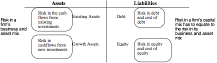
As
with any other aspect of the balance sheet, this one has to balance has well,
with the weighted risk in the assets being equal to the weighted risk in the
ingredients to capital – debt and equity. Note that the risk in the
equity investment in a business is partly determined by the risk of the
business the firm is in and partly by its choice on how much debt to use to
fund that business. The equity in a safe business can be rendered risky, if the
firm uses enough debt to fund that business.
In
discount rate terms, the risk in the equity in a business is measured with the
cost of equity, whereas the risk in the business is captured in the cost of
capital. The latter will be a weighted average of the cost of equity and the
cost of debt, with the weights reflecting the proportional use of each source
of funding.
Measuring Equity
Risk and the Cost of Equity
Measuring
the risk in equity investments and converting that risk measure into a cost of
equity is rendered difficult by two factors. The first is that equity has an
implicit cost, which is unobservable, unlike debt, which comes with an explicit
cost in the form of an interest rate. The second is that risk in the eyes of
the beholder and different equity investors in the same business can have very
different perceptions of risk in that business and demand different expected
returns as a consequence.
The Diversified Marginal Investor
If
there were only one equity investor in a company, estimating equity risk and
the cost of equity would be a far simpler exercise. We would measure the risk
of investing in equity in that company to the investor and assess a reasonable
rate of return, given that risk. In a publicly traded company, we run into the
practical problem that the equity investors number in the hundreds, if not the
thousands, and that they not only vary in size, from small to large investors,
but also in risk aversion. So, whose perspective should we take when measuring
risk and cost of equity? In corporate finance and valuation, we develop the
notion of the marginal investor,
i.e., the investor most likely to influence the market price of publicly traded
equity. The marginal investor in a publicly traded stock has to own enough
stock in the company to make a difference and be willing to trade on that
stock. The common theme shared by risk and return models in finance is that the
marginal investor is diversified, and we measure the risk in an investment as
the risk added to a diversified portfolio.
Put another way, it is only that portion of the risk in an investment
that is attributable to the broader market or economy, and hence not
diversifiable, that should be built into expected returns.
Models for Expected Return (Cost of Equity)
It
is on the issue of how best to measure this non-diversifiable risk that the
different risk and return models in finance part ways. Let use consider the
alternatives:
·
In the capital
asset pricing model (CAPM), this risk is captured in the beta that we assign an asset/business,
with that number carrying the burden of measuring exposure to all of the
components of market risk. The expected return on an investment can then be
specified as a function of three variables – the riskfree rate, the beta
of the investment and the equity risk premium (the premium demanded for
investing in the average risk investment):
Expected
Return = Riskfree Rate + BetaInvestment
(Equity Risk Premium)
The riskfree rate and equity risk
premium are the same for all investments in a market but the beta will capture
the market risk exposure of the investment; a beta of one represents an average
risk investment, and betas above (below) one indicate investments that are
riskier (safer) than the average risk investment in the market.
·
In the arbitrage pricing and multi-factor
models, we allow for multiple sources of non-diversifiable (or market) risk and
estimate betas against each one. The expected return on an investment can be
written as a function of the multiple betas (relative to each market risk
factor) and the risk premium for that factor. If there are k factors in the
model with bji
and Risk Premiumj representing the beta
and risk premium of factor j, the expected return on the investment can be
written as:
Expected
Return = ![]()
Note
that the capital asset pricing model can be written as a special case of these
multi-factor models, with a single factor (the market) replacing the multiple
factors.
·
The final class of models can be categorized as
proxy models. In these models, we essentially give up on measuring risk
directly and instead look at historical data for clues on what types of
investments (stocks) have earned high returns in the past, and then use the
common characteristic(s) that they share as a measure of risk. For instance,
researchers have found that market capitalization and price to book ratios are
correlated with returns; stocks with small market capitalization and low price
to book ratios have historically earned higher returns than large market stocks
with higher price to book ratios. Using the historical data, we can then
estimate the expected return for a company, based on its market capitalization
and price to book ratio.
Expected
Return = a + b(Market Capitalization) + c (Price to
Book Ratio)
Since
we are no longer working within the confines of an economic model, it is not
surprising that researchers keep finding new variables (trading volume, price
momentum) that improve the predictive power of these models. The open question,
though, is whether these variables are truly proxies for risk or indicators of
market inefficiency. In effect, we may be explaining away the misvaluatiion of classes of stock by the market by using
proxy models for risk.
Estimation Issues
With
the CAPM and multi-factor models, the inputs that we need for the expected
return are straightforward. We need to come up with a risk free rate and an
equity risk premium (or premiums in the multi-factor models) to use across all
investments. Once we have these market-wide estimates, we then have to measure
the risk (beta or betas) in individual investments. In this section, we will lay out the broad principles that will govern these
estimates but we will return in future chapters to the details of how best to
make these estimates for different types of businesses:
·
The riskfree rate is the expected return on an
investment with guaranteed returns; in effect, you expected return is also your
actual return. Since the return is guaranteed, there are two conditions that an
investment has to meet to be riskfree. The first is that the entity making the
guarantee has to have no default risk; this is why we use government securities
to derive riskfree rates, a necessary though not always a sufficient condition.
As we will see in chapter 6, there is default risk in many government
securities that is priced into the expected return. The second is that the time
horizon matters. A six-month treasury bill is not riskfree, if you are looking
at a five-year time horizon, since we are exposed to reinvestment risk. In
fact, even a 5-year treasury bond may not be riskless, since the coupons
received every six months have to be reinvested. Clearly, getting a riskfree
rate is not as simple as it looks at the outset.
·
The equity risk premium is the premium that
investors demand for investing in risky assets (or equities) as a class,
relative to the riskfree rate. It will be a function not only of how much risk
investors perceive in equities, as a class, but the risk aversion that they
bring to the market. It also follows that the equity risk premium can change
over time, as market risk and risk aversion both change. The conventional
practice for estimating equity risk premiums is to use the historical risk
premium, i.e., the premium investors have earned over long periods (say 75
years) investing in equities instead of riskfree (or close to riskfree) investments.
In chapter 7, we will question the efficacy of this process and offer
alternatives.
·
To estimate the beta in the CAPM and betas in
multi-factor models, we draw on statistical techniques and historical data. The
standard approach for estimating the CAPM beta is to run a regression of
returns on a stock against returns on a broad equity market index, with the
slope capturing how much the stock moves, for any given market move. To
estimate betas in the arbitrage pricing model, we use
historical return data on stocks and factor analysis to extract both the number
of factors in the models, as well as factor betas for individual companies. As
a consequence, the beta estimates that we obtain will always be backward
looking (since they are derived from past data) and noisy (they are statistical
estimates, with standard errors). In addition, these approaches clearly will
not work for investments that do not have a trading history (young companies,
divisions of publicly traded companies). One solution is to replace the
regression beta with a bottom-up beta,
i.e., a beta that is based upon industry averages for the businesses that the
firm is in, adjusted for differences in financial leverage.[1]
Since industry averages are more precise than individual regression betas, and
the weights on the businesses can reflect the current mix of a firm, bottom up
betas generally offer better estimates for the future.
The Cost of Debt
While
equity investors receive residual cash flows and bear the bulk of the operating
risk in most firms, lenders to the firm also face the risk that they will not
receive their promised payments – interest expenses and principal
repayments. It is to cover this default risk that lenders add a “default spread”
to the riskless rate when they lend money to firms; the greater the perceived
risk of default, the greater the default spread and the cost of debt. The other
dimension on which debt and equity can vary is in their treatment for tax
purposes, with cashflows to equity investors (dividends and stock buybacks)
coming from after-tax cash flows, whereas interest payments are tax
deductible. In effect, the tax law
provides a benefit to debt and lowers the cost of borrowing to businesses.
To
estimate the cost of debt for a firm, we need three components. The first is
the riskfree rate, an input to the cost of equity as well. As a general rule,
the riskfree rate used to estimate the cost of equity should be used to compute
the cost of debt as well; if the cost of equity is based upon a long-term
riskfree rate, as it often is, the cost of debt should be based upon the same
rate. The second is the default spread and there are three approaches that are
used, depending upon the firm being analyzed.
·
If the firm has traded bonds outstanding, the
current market interest rate on the bond (yield to maturity) is used as the
cost of debt. This is appropriate only if the bond is liquid and is
representative of the overall debt of the firm; even risky firms can issue safe
bonds, backed up by the most secure assets of the firms.
·
If the firm has a bond rating from an
established ratings agency such as S&P or Moody’s, we can estimate a
default spread based upon the rating. In September 2008, for instance, the
default spread for BBB rated bonds was 2% and would have been used as the
spread for any BBB rated company.
·
If the firm is unrated and has debt outstanding
(bank loans), we can estimate a “synthetic” rating for the firm, based upon its
financial ratios. A simple, albeit effective approach for estimating the
synthetic ratio is to base it entirely on the interest coverage ratio (EBIT/
Interest expense) of a firm; higher interest coverage ratios will yield higher
ratings and lower interest coverage ratios.
The
final input needed to estimate the cost of debt is the tax rate. Since interest
expenses save you taxes at the margin, the tax rate that is relevant for this
calculation is not the effective tax rate but the marginal tax rate. In the
United States, where the federal corporate tax rate is 35% and state and local
taxes add to this, the marginal tax rate for corporations in 2008 was close to
40%, much higher than the average effective tax rate, across companies, of 28%.
The after-tax cost of debt for a firm is therefore:
After-tax
cost of debt = (Riskfree Rate + Default Spread) (1- Marginal tax rate)
The
after-tax cost of debt for most firms will be significantly lower than the cost
of equity for two reasons. First, debt in a firm is generally less risky than
its equity, leading to lower expected returns. Second, there is a tax saving
associated with debt that does not exist with equity.
Debt Ratios and
the Cost of Capital
Once
we have estimated the costs of debt and equity, we still have to assign weights
for the two ingredients. To come up with this value, we could start with the
mix of debt and equity that the firm uses right now. In making this estimate,
the values that we should use are market values, rather than book values. For
publicly traded firms, estimating the market value of equity is usually a
trivial exercise, where we multiply the share price by the number of shares
outstanding. Estimating the market value of debt is usually a more difficult
exercise, since most firms have some debt that is not traded. Though many
practitioners fall back on book value of debt as a proxy of market value,
estimating the market value of debt is still a better practice.
Once we have the current market value weights for debt and equity for use in the cost of capital, we have a follow up judgment to make in terms of whether these weights will change or remain stable. If we assume that they will change, we have to specify both what the right or target mix for the firm will be and how soon the change will occur. In an acquisition, for instance, we can assume that the acquirer can replace the existing mix with the target mix instantaneously. As passive investors in publicly traded firms, we have to be more cautious, since we do not control how a firm funds its operations. In this case, we may adjust the debt ratio from the current mix to the target over time, with concurrent changes in the costs of debt, equity and capital. In fact, the last point about debt ratios and costs of capital changing over time is worth reemphasizing. As companies change over time, we should expect the cost of capital to change as well.