 The
Little Book of Valuation
The
Little Book of Valuation
The Mechanics of Time Value
The
process of discounting future cash flows converts them into cash flows in
present value terms. Conversely, the process of compounding converts present
cash flows into future cash flows. There are five types of cash
flows—simple cash flows, annuities, growing annuities, perpetuities, and
growing perpetuities—which we discuss next.
Simple Cash Flows
A
simple cash flow is a single cash flow in a specified future time period; it
can be depicted on a time line as in Figure A3.3.
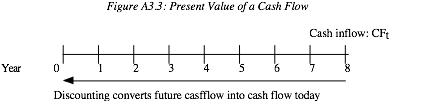
where CFt = the cash flow at time t.
This
cash flow can be discounted back to the present using a discount rate that
reflects the uncertainty of the cash flow. Concurrently, cash flows in the
present can be compounded to arrive at an expected future cash flow.
Discounting
a cash flow converts it into present value dollars and enables the user to do
several things. First, once cash flows are converted into present value
dollars, they can be aggregated and compared. Second, if present values are
estimated correctly, the user should be indifferent between the future cash
flow and the present value of that cash flow. The present value of a cash flow
can be written as follows
Present
Value of Simple Cash Flow = ![]()
where r = discount rate.
Other
things remaining equal, the present value of a cash flow will decrease as the
discount rate increases and continue to decrease the further into the future
the cash flow occurs.
Current
cash flows can be moved to the future by compounding the cash flow at the
appropriate discount rate.
Future
Value of Simple Cash Flow = CF0 (1 + r)t
where CF0
= cash flow now, r = discount rate.
Again, the compounding effect increases with both the discount rate and the
compounding period.
The
frequency of compounding affects both the future and present values of cash
flows. In the examples just discussed, the cash flows were
assumed to be discounted and compounded annually—that is, interest
payments and income were computed at the end of each year, based on the balance
at the beginning of the year. In some cases, however, the interest may be
computed more frequently, such as on a monthly or semi-annual basis. In these
cases, the present and future values may be very different from those computed
on an annual basis; the stated interest rate on an annual basis can deviate
significantly from the effective or true interest rate. The effective interest
rate can be computed as follows:
Effective
Interest Rate = ![]()
where n = number of compounding periods during
the year (2 = semi-annual; 12 = monthly). For instance, a 10 percent annual
interest rate, if there is semi-annual compounding, works out to an effective
interest rate of
Effective
Interest Rate = 1.052
– 1 = 0.10125 or 10.125%
As compounding becomes continuous,
the effective interest rate can be computed as follows
Effective
Interest Rate = expr – 1
where exp
= exponential function and r = stated
annual interest rate. Table A3.2 provides the effective rates as a function of
the compounding frequency.
Table A3.2 Effect of Compounding Frequency
on Effective Interest Rates
|
Frequency
|
Rate |
t (Days) |
Formula |
Effective
Annual Rate |
|
Annual |
10% |
1 |
0.10 |
10% |
|
Semi-annual |
10% |
2 |
(1 + 0.10/2)2
– 1 |
10.25% |
|
Monthly |
10% |
12 |
(1 + 0.10/12)12
– 1 |
10.47% |
|
Daily |
10% |
365 |
(1 + 0.10/365)365
– 1 |
10.5156% |
|
Continuous |
10% |
|
exp0.10 – 1 |
10.5171% |
As you can see, compounding becomes
more frequent, the effective rate increases, and the present value of future
cash flows decreases.
Annuities
An
annuity is a constant cash flow that
occurs at regular intervals for a fixed period of time. Defining A to be the
annuity, the time line for an annuity may be drawn as follows:
A A A A
| | | |
0 1 2 3 4
An
annuity can occur at the end of each period, as in this time line, or at the
beginning of each period.
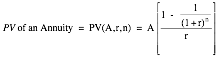
where A = annuity, r
= discount rate, and n = number of
years. Accordingly, the notation we will use in the rest of this book for the
present value of an annuity will be PV(A,r,n).
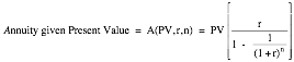
Individuals or businesses who
have a fixed obligation to meet or a target to meet (in terms of savings) some
time in the future need to know how much they should set aside each period to
reach this target. If you are given the future value and are looking for an
annuity—A(FV,r,n) in terms of notation:
![]()
The
annuities considered thus far i are end-of-the-period cash
flows. Both the present and future values will be affected if the cash flows
occur at the beginning of each period instead of the end. To illustrate this
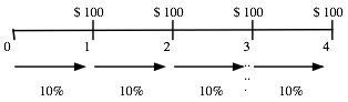
effect, consider an annuity of $100 at the end of each year for the next four
years, with a discount rate of 10 percent.
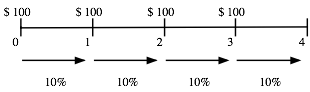
Contrast this with an annuity of
$100 at the beginning of each year for the next four years, with the same
discount rate.
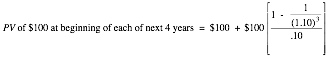
Because the first of these
annuities occurs right now and the remaining cash flows take the form of an
end-of-the-period annuity over three years, the present value of this annuity
can be written as follows:
In general, the present value of a
beginning-of-the-period annuity over n
years can be written as follows:
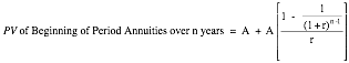
This
present value will be higher than the present value of an equivalent annuity at
the end of each period.
Growing Annuities
A
growing annuity is a cash flow that
grows at a constant rate for a specified period of time. If A is the current
cash flow, and g is the expected growth
rate, the time line for a growing annuity appears as follows:
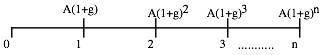
Note that to qualify as a growing
annuity, the growth rate in each period has to be the same as the growth rate
in the prior period.
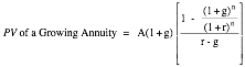
In
most cases, the present value of a growing annuity can be estimated by using
the following formula:
The present value of a growing
annuity can be estimated in all cases, but one—where the growth rate is
equal to the discount rate. In that case, the present value is equal to the
nominal sums of the annuities over the period, without the growth effect.
PV
of a Growing Annuity for n Years
(when r = g) = nA
Note also that this formulation
works even when the growth rate is greater than the discount rate.[2]
Perpetuities
A perpetuity is a
constant cash flow at regular intervals forever. The present value of a perpetuity can be written as
![]()
where A is the perpetuity.
A
growing perpetuity is a cash flow
that is expected to grow at a constant rate forever. The present value of a
growing perpetuity can be written as:
![]()
where CF1 is
the expected cash flow next year, g
is the constant growth rate, and r is
the discount rate. Although a growing perpetuity and a growing annuity share
several features, the fact that a growing perpetuity lasts forever puts
constraints on the growth rate. It has to be less than the discount rate for
this formula to work.