The Little Book of Valuation

Terminal Value

Publicly traded firms do not have finite lives. Given that we cannot estimate cash flows forever, we generally impose closure in valuation models by stopping our estimation of cash flows sometime in the future and then computing a terminal value that reflects all cash flows beyond that point. There are three approaches generally used to estimate the terminal value. The most common approach, which is to apply a multiple to earnings in the terminal year to arrive at the terminal value, is inconsistent with intrinsic valuation. Since these multiples are usually obtained by looking at what comparable firms are trading at in the market today, this is a relative valuation, rather than a discounted cash flow valuation. The two more legitimate ways of estimating terminal value are to estimate a liquidation value for the assets of the firm, assuming that the assets are sold in the terminal year, and the other is to estimate a going concern or a terminal value.

1. Liquidation Value

If we assume that the business will be ended in the terminal year and that its assets will be liquidated at that time, we can estimate the proceeds from the liquidation. This liquidation value still has to be estimated, using a combination of market-based numbers (for assets that have ready markets) and cashflow-based estimates. For firms that have finite lives and marketable assets (like real estate), this represents a fairly conservative way of estimating terminal value. For other firms, estimating liquidation value becomes more difficult to do, either because the assets are not separable (brand name value in a consumer product company) or because there is no market for the individual assets. One approach is to use the estimated book value of the assets as a starting point, and to estimate the liquidation value, based upon the book value.

2. Going Concern or Terminal value

If we treat the firm as a going concern at the end of the estimation period, we can estimate the value of that concern by assuming that cash flows will grow at a constant rate forever afterwards. This perpetual growth model draws on a simple present value equation to arrive at terminal value:

Our definitions of cash flow and growth rate have to be consistent with whether we are valuing dividends, cash flows to equity or cash flows to the firm; the discount rate will be the cost of equity for the first two and the cost of capital for the last. The perpetual growth model is a powerful one, but it can be easily misused. In fact, analysts often use it is as a piggy bank that they go to whenever they feel that the value that they have derived for an asset is too low or high. Small changes in the inputs can alter the terminal value dramatically. Consequently, there are three key constraints that should be imposed on its estimation:

a. Cap the growth rate: Small changes in the stable growth rate can change the terminal value significantly and the effect gets larger as the growth rate approaches the discount rate used in the estimation. The fact that a stable growth rate is constant forever, however, puts strong constraints on how high it can be. Since no firm can grow forever at a rate higher than the growth rate of the economy in which it operates, the constant growth rate cannot be greater than the overall growth rate of the economy. So, what is the maximum stable growth rate that you can use in a valuation? The answer will depend on whether the valuation is being done in real or nominal terms, and if the latter, the currency used to estimate cash flows. With the former, you would use the real growth rate in the economy as your constraint, whereas with the latter, you would add expected inflation in the currency to the real growth. Setting the stable growth rate to be less than or equal to the growth rate of the economy is not only the consistent thing to do but it also ensures that the growth rate will be less than the discount rate. This is because of the relationship between the riskless rate that goes into the discount rate and the growth rate of the economy. Note that the riskless rate can be written as:

Nominal riskless rate = Real riskless rate + Expected inflation rate

In the long term, the real riskless rate will converge on the real growth rate of the economy and the nominal riskless rate will approach the nominal growth rate of the economy. In fact, a simple rule of thumb on the stable growth rate is that it should not exceed the riskless rate used in the valuation.

b. Use mature company risk characteristics: As firms move from high growth to stable growth, we need to give them the characteristics of stable growth firms. A firm in stable growth is different from that same firm in high growth on a number of dimensions. In general, you would expect stable growth firms to be less risky and use more debt. In practice, we should move betas for even high risk firms towards one in stable growth and give them debt ratios, more consistent with larger, more stable cashflows.

c. Reinvestment and Excess Return Assumptions: Stable growth firms tend to reinvest less than high growth firms and it is critical that we both capture the effects of lower growth on reinvestment and that we ensure that the firm reinvests enough to sustain its stable growth rate in the terminal phase. Given the relationship between growth, reinvestment rate and returns that we established in the section on expected growth rates, we can estimate the reinvestment rate that is consistent with expected growth :

In the dividend discount model:

In the FCFE model:

In the FCFF model:

Linking the reinvestment rate and retention ratio to the stable growth rate also makes the valuation less sensitive to assumptions about stable growth. While increasing the stable growth rate, holding all else constant, can dramatically increase value, changing the reinvestment rate as the growth rate changes will create an offsetting effect.

The gains from increasing the growth rate will be partially or completely offset by the loss in cash flows because of the higher reinvestment rate. Whether value increases or decreases as the stable growth increases will entirely depend upon what you assume about excess returns. If the return on capital is higher than the cost of capital in the stable growth period, increasing the stable growth rate will increase value. If the return on capital is equal to the stable period cost of capital, increasing the stable growth rate will have no effect on value. Substituting in the stable growth rate as a function of the reinvestment rate, from above, you get:

Setting the return on capital equal to the cost of capital, you arrive at:

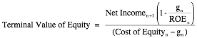
You could establish the same propositions with equity income and cash flows and show that the terminal value of equity is a function of the difference between the return on equity and cost of equity.

In closing, the key assumption in the terminal value computation is not what growth rate you use in the valuation, but what excess returns accompany that growth rate. If you assume no excess returns, the growth rate becomes irrelevant. There are some valuation experts who believe that this is the only sustainable assumption, since no firm can maintain competitive advantages forever. In practice, though, there may be some wiggle room, insofar as the firm may become a stable growth firm before its excess returns go to zero. If that is the case and the competitive advantages of the firm are strong and sustainable (even if they do not last forever), we may be able to give the firm some excess returns in perpetuity. As a simple rule of thumb again, these excess returns forever should be modest (<4-5%) and will affect the terminal value.