Statistical Distributions
Every
statistics book provides a listing of statistical distributions, with their
properties, but browsing through these choices can be frustrating to anyone
without a statistical background, for two reasons. First, the choices seem
endless, with dozens of distributions competing for your attention, with little
or no intuitive basis for differentiating between them. Second, the descriptions
tend to be abstract and emphasize statistical properties such as the moments,
characteristic functions and cumulative distributions. In this appendix, we
will focus on the aspects of distributions that are most useful when analyzing
raw data and trying to fit the right distribution to that data.
Fitting the Distribution
When
confronted with data that needs to be characterized by a distribution, it is
best to start with the raw data and answer four basic questions about the data
that can help in the characterization. The first relates to whether the data
can take on only discrete values or whether the data is continuous;
whether a new pharmaceutical drug gets FDA approval or not is a discrete value
but the revenues from the drug represent a continuous variable. The second
looks at the symmetry of the data and if there is asymmetry, which
direction it lies in; in other words, are positive and negative outliers
equally likely or is one more likely than the other. The third question is
whether there are upper or lower limits on the data;; there are some
data items like revenues that cannot be lower than zero whereas there are
others like operating margins that cannot exceed a value (100%). The final and related
question relates to the likelihood of observing extreme values in the
distribution; in some data, the extreme values occur very infrequently whereas
in others, they occur more often.
Is the data discrete or continuous?
The
first and most obvious categorization of data should be on whether the data is
restricted to taking on only discrete values or if it is continuous. Consider
the inputs into a typical project analysis at a firm. Most estimates that go
into the analysis come from distributions that are continuous; market size,
market share and profit margins, for instance, are all continuous variables.
There are some important risk factors, though, that can take on only discrete
forms, including regulatory actions and the threat of a terrorist attack; in
the first case, the regulatory authority may dispense one of two or more
decisions which are specified up front and in the latter, you are subjected to
a terrorist attack or you are not.
With
discrete data, the entire distribution can either be developed from scratch or
the data can be fitted to a pre-specified discrete distribution. With the
former, there are two steps to building the distribution. The first is
identifying the possible outcomes and the second is to estimate probabilities
to each outcome. As we noted in the text, we can draw on historical data or
experience as well as specific knowledge about the investment being analyzed to
arrive at the final distribution. This
process is relatively simple to accomplish when there are a few outcomes with a
well-established basis for estimating probabilities but becomes more tedious as
the number of outcomes increases. If it is difficult or impossible to build up
a customized distribution, it may still be possible fit the data to one of the
following discrete distributions:
a.
Binomial distribution: The binomial distribution
measures the probabilities of the number of successes over a given number of
trials with a specified probability of success in each try. In the simplest
scenario of a coin toss (with a fair coin), where the probability of getting a
head with each toss is 0.50 and there are a hundred trials, the binomial
distribution will measure the likelihood of getting anywhere from no heads in a
hundred tosses (very unlikely) to 50 heads (the most likely) to 100 heads (also
very unlikely). The binomial distribution in this case will be symmetric,
reflecting the even odds; as the probabilities shift from even odds, the
distribution will get more skewed. Figure 6A.1 presents binomial distributions
for three scenarios – two with 50% probability of success and one with a
70% probability of success and different trial sizes.
Figure
6A.1: Binomial Distribution
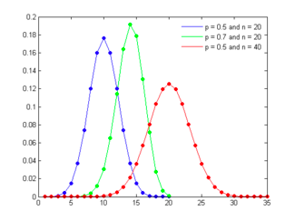
As the
probability of success is varied (from 50%) the distribution will also shift
its shape, becoming positively skewed for probabilities less than 50% and
negatively skewed for probabilities greater than 50%.[1]
b.
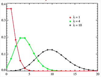
Poisson distribution: The Poisson distribution measures
the likelihood of a number of events occurring within a given time interval,
where the key parameter that is required is the average number of events in the
given interval (l). The resulting
distribution looks similar to the binomial, with the skewness being positive
but decreasing with l. Figure 6A.2 presents three Poisson
distributions, with l ranging from 1 to
10.
Figure
6A.2: Poisson Distribution
c.
Negative Binomial distribution: Returning again to the
coin toss example, assume that you hold the number of successes fixed at a
given number and estimate the number of tries you will have before you reach
the specified number of successes. The resulting distribution is called the
negative binomial and it very closely resembles the Poisson. In fact, the
negative binomial distribution converges on the Poisson distribution, but will
be more skewed to the right (positive values) than the Poisson distribution
with similar parameters.
d.
Geometric distribution: Consider again the coin toss
example used to illustrate the binomial. Rather than focus on the number of
successes in n trials, assume that you were measuring the likelihood of when
the first success will occur. For instance, with a fair coin toss, there is
a 50% chance that the first success will occur at the first try, a 25% chance
that it will occur on the second try and a 12.5% chance that it will occur on
the third try. The resulting distribution is positively skewed and looks as
follows for three different probability scenarios (in figure 6A.3):
Figure
6A.3: Geometric Distribution
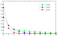
Note that the distribution is
steepest with high probabilities of success and flattens out as the probability
decreases. However, the distribution is always positively skewed.
e.
Hypergeometric distribution: The hypergeometric
distribution measures the probability of a specified number of successes in n
trials, without replacement, from a finite population. Since the
sampling is without replacement, the probabilities can change as a function of
previous draws. Consider, for instance, the possibility of getting four face
cards in hand of ten, over repeated draws from a pack. Since there are 16 face
cards and the total pack contains 52 cards, the probability of getting four
face cards in a hand of ten can be estimated. Figure 6A.4 provides a graph of
the hypergeometric distribution:
Figure
6A.4: Hypergeometric Distribution
Note
that the hypergeometric distribution converges on binomial distribution as the
as the population size increases.
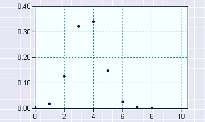
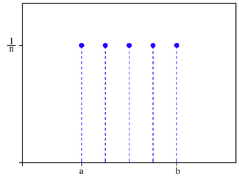
f. Discrete
uniform distribution: This is the simplest of discrete distributions and
applies when all of the outcomes have an equal probability of occurring. Figure 6A.5 presents a uniform discrete
distribution with five possible outcomes, each occurring 20% of the time:
Figure
6A.5: Discrete Uniform Distribution
The discrete uniform distribution is best reserved for
circumstances where there are multiple possible outcomes, but no information
that would allow us to expect that one outcome is more likely than the others.
With continuous data, we cannot
specify all possible outcomes, since they are too numerous to list, but we have
two choices. The first is to convert the continuous data into a discrete form
and then go through the same process that we went through for discrete
distributions of estimating probabilities. For instance, we could take a
variable such as market share and break it down into discrete blocks –
market share between 3% and 3.5%, between 3.5% and 4% and so on – and
consider the likelihood that we will fall into each block. The second is to
find a continuous distribution that best fits the data and to specify the
parameters of the distribution. The rest of the appendix will focus on how to
make these choices.
How symmetric is the data?
There are some datasets that
exhibit symmetry, i.e., the upside is mirrored by the downside. The symmetric
distribution that most practitioners have familiarity with is the normal
distribution, sown in Figure 6A.6, for a range of parameters:
Figure 6A.6: Normal Distribution
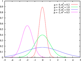
The normal distribution has several features that make it
popular. First, it can be fully characterized by just two parameters –
the mean and the standard deviation – and thus reduces estimation pain.
Second, the probability of any value occurring can be obtained simply by
knowing how many standard deviations separate the value from the mean; the probability
that a value will fall 2 standard deviations from the mean is roughly 95%. The normal distribution is best
suited for data that, at the minimum, meets the following conditions:
- There
is a strong tendency for the data to take on a central value.
- Positive
and negative deviations from this central value are equally likely
- The
frequency of the deviations falls off rapidly as we move further away from
the central value.
The last two conditions show up when we compute the
parameters of the normal distribution: the symmetry of deviations leads to zero
skewness and the low probabilities of large deviations from the central value
reveal themselves in no kurtosis.
There is a cost we pay, though,
when we use a normal distribution to characterize data that is non-normal since
the probability estimates that we obtain will be misleading and can do more
harm than good. One obvious problem is when the data is asymmetric but another potential
problem is when the probabilities of large deviations from the central value do
not drop off as precipitously as required by the normal distribution. In
statistical language, the actual distribution of the data has fatter tails than
the normal. While all of symmetric distributions in the family are like the
normal in terms of the upside mirroring the downside, they vary in terms of
shape, with some distributions having fatter tails than the normal and the others
more accentuated peaks. These
distributions are characterized as leptokurtic and you can consider two
examples. One is the logistic distribution, which has longer tails and a higher
kurtosis (1.2, as compared to 0 for the normal distribution) and the other are
Cauchy distributions, which also exhibit symmetry and higher kurtosis and are
characterized by a scale variable that determines how fat the tails are. Figure
6A.7 present a series of Cauchy distributions that exhibit the bias towards
fatter tails or more outliers than the normal distribution.
Figure 6A.7: Cauchy Distribution

Either the logistic or the Cauchy distributions can be used
if the data is symmetric but with extreme values that occur more frequently
than you would expect with a normal distribution.
As the probabilities of extreme
values increases relative to the central value, the distribution will flatten
out. At its limit, assuming that the data stays symmetric and we put limits on
the extreme values on both sides, we end up with the uniform distribution,
shown in figure 6A.8:
Figure 6A.8: Uniform Distribution
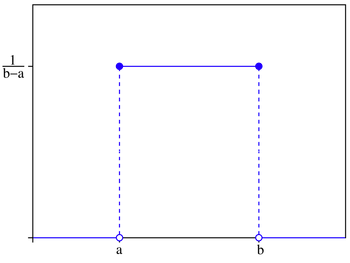
When is it appropriate to assume a uniform distribution for
a variable? One possible scenario is when you have a measure of the highest and
lowest values that a data item can take but no real information about where
within this range the value may fall. In other words, any value within that
range is just as likely as any other value.
Most data does not exhibit symmetry
and instead skews towards either very large positive or very large negative
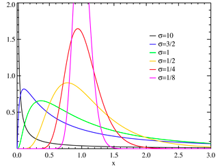
values. If the data is positively skewed, one common choice is the lognormal
distribution, which is typically characterized by three parameters: a shape (s or sigma),
a scale (m or median) and a shift
parameter (![]() ). When m=0 and
). When m=0 and ![]() =1, you have the standard lognormal distribution and
when
=1, you have the standard lognormal distribution and
when ![]() =0, the distribution requires only scale and sigma
parameters. As the sigma rises, the peak of the distribution shifts to the left
and the skewness in the distribution increases. Figure 6A.9 graphs lognormal
distributions for a range of parameters:
=0, the distribution requires only scale and sigma
parameters. As the sigma rises, the peak of the distribution shifts to the left
and the skewness in the distribution increases. Figure 6A.9 graphs lognormal
distributions for a range of parameters:
Figure 6A.9: Lognormal distribution
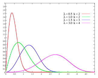
The Gamma and Weibull distributions are two distributions
that are closely related to the lognormal distribution; like the lognormal
distribution, changing the parameter levels (shape, shift and scale) can cause
the distributions to change shape and become more or less skewed. In all of
these functions, increasing the shape parameter will push the distribution
towards the left. In fact, at high values of sigma, the left tail disappears entirely
and the outliers are all positive. In this form, these distributions all
resemble the exponential, characterized by a location (m) and scale parameter
(b), as is clear from figure 6A.10.
Figure
6A.10: Weibull Distribution
The question of which of these distributions will best fit
the data will depend in large part on how severe the asymmetry in the data is. For
moderate positive skewness, where there are both positive and negative
outliers, but the former and larger and more common, the standard lognormal
distribution will usually suffice. As the skewness becomes more severe, you may
need to shift to a three-parameter lognormal distribution or a Weibull
distribution, and modify the shape parameter till it fits the data. At the
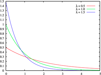
extreme, if there are no negative outliers and the only positive outliers in
the data, you should consider the exponential function, shown in Figure 6a.11:
Figure
6A.11: Exponential Distribution
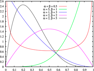
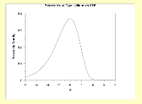
If
the data exhibits negative slewness, the choices of distributions are more
limited. One possibility is the Beta distribution, which has two shape
parameters (p and q) and upper and lower bounds on the data (a and b). Altering
these parameters can yield distributions that exhibit either positive or
negative skewness, as shown in figure 6A.12:
Figure
6A.12: Beta Distribution
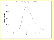
Another is an extreme value distribution, which can also be
altered to generate both positive and negative skewness, depending upon whether
the extreme outcomes are the maximum (positive) or minimum (negative) values
(see Figure 6A.13)
Figure 6A.13:
Extreme Value Distributions
Are there upper or lower limits on data values?
There
are often natural limits on the values that data can take on. As we noted
earlier, the revenues and the market value of a firm cannot be negative and the
profit margin cannot exceed 100%. Using a distribution that does not constrain
the values to these limits can create problems. For instance, using a normal
distribution to describe profit margins can sometimes result in profit margins
that exceed 100%, since the distribution has no limits on either the downside
or the upside.
When
data is constrained, the questions that needs to be answered are whether the
constraints apply on one side of the distribution or both, and if so, what the
limits on values are. Once these questions have been answered, there are two
choices. One is to find a continuous distribution that conforms to these
constraints. For instance, the lognormal distribution can be used to model
data, such as revenues and stock prices that are constrained to be never less
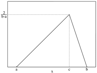
than zero. For data that have both upper and lower limits, you could use the
uniform distribution, if the probabilities of the outcomes are even across
outcomes or a triangular distribution (if the data is clustered around a
central value). Figure 6A.14 presents a triangular distribution:
Figure
6A.14: Triangular Distribution
An alternative approach is to use a continuous distribution that
normally allows data to take on any value and to put upper and lower limits on
the values that the data can assume. Note that the cost of putting these
constrains is small in distributions like the normal where the probabilities of
extreme values is very small, but increases as the distribution exhibits fatter
tails.
How likely are you to see extreme values of data, relative to the middle
values?
As
we noted in the earlier section, a key consideration in what distribution to
use to describe the data is the likelihood of extreme values for the data,
relative to the middle value. In the case of the normal distribution, this
likelihood is small and it increases as you move to the logistic and Cauchy
distributions. While it may often be more realistic to use the latter to
describe real world data, the benefits of a better distribution fit have to be
weighed off against the ease with which parameters can be estimated from the
normal distribution. Consequently, it may make sense to stay with the normal
distribution for symmetric data, unless the likelihood of extreme values
increases above a threshold.
The
same considerations apply for skewed distributions, though the concern will
generally be more acute for the skewed side of the distribution. In other
words, with positively skewed distribution, the question of which distribution
to use will depend upon how much more likely large positive values are than
large negative values, with the fit ranging from the lognormal to the
exponential.
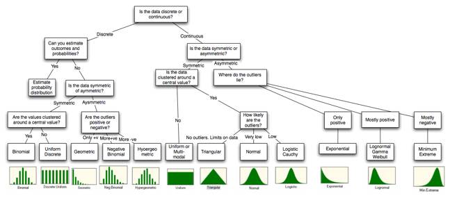
In
summary, the question of which distribution best fits data cannot be answered
without looking at whether the data is discrete or continuous, symmetric or
asymmetric and where the outliers lie. Figure 6A.15 summarizes the choices in a
chart.
Tests for Fit
The
simplest test for distributional fit is visual with a comparison of the
histogram of the actual data to the fitted distribution. Consider figure 6A.16,
where we report the distribution of current price earnings ratios for US stocks
in early 2007, with a normal distribution superimposed on it.
Figure 6A.16:
Current PE Ratios for US Stocks – January 2007
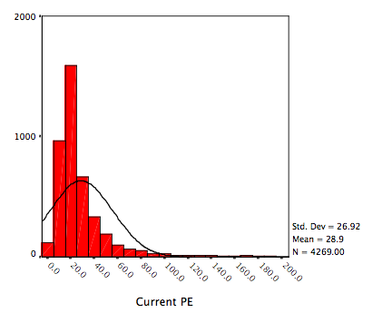
The distributions are so clearly divergent that the normal
distribution assumption does not hold up.
A
slightly more sophisticated test is to compute the moments of the actual data
distribution – the mean, the standard deviation, skewness and kurtosis
– and to examine them for fit to the chosen distribution. With the
price-earnings data above, for instance, the moments of the distribution and
key statistics are summarized in
table 6A.1:
Table 6A.1: Current
PE Ratio for US stocks – Key Statistics
|
|
Current
PE |
Normal
Distribution |
|
|||
|
Mean |
28.947 |
|
|
|||
|
Median |
20.952 |
Median
= Mean |
|
|||
|
Standard
deviation |
26.924 |
|
|
|||
|
Skewness |
3.106 |
0 |
|
|||
|
Kurtosis |
11.936 |
0 |
|
|||
|
|
|
||||
|
|
|
||||
|
|
|
||||
|
|
|
||||
|
|
|
||||
|
|
|
||||
|
|
|
||||
|
|
|
||||
|
|
|
||||
|
|
|
||||
|
|
|
||||
|
|
|
||||
|
|
|
||||
|
|
|
||||
|
||||||
Since the normal distribution has no skewness
and zero kurtosis, we can easily reject the hypothesis that price
earnings ratios are normally distributed.
The typical tests for
goodness of fit compare the actual distribution function of the
data with the cumulative distribution function of the
distribution that is being used to characterize the data, to
either accept the hypothesis that the chosen distribution fits
the data or to reject it. Not surprisingly, given its constant
use, there are more tests for normality than for any other
distribution. The Kolmogorov-Smirnov test is one of the oldest tests
of fit for distributions[2],
dating back to 1967. Improved versions of the tests include the
Shapiro-Wilk and Anderson-Darling tests. Applying these tests to
the current PE ratio yields the unsurprising result that the
hypothesis that current PE ratios are drawn from a normal
distribution is roundly rejected:
Tests of Normality

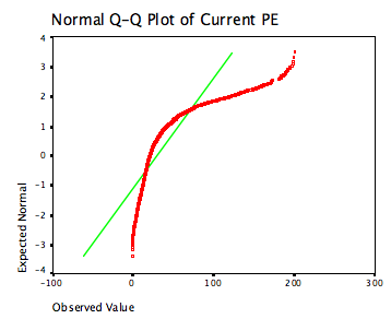
There are graphical tests of normality,
where probability plots can be used to assess the hypothesis that
the data is drawn from a normal distribution. Figure 6A.17
illustrates this, using current PE ratios as the data set.
|
|
|
|
|
Given that the normal distribution is one of
easiest to work with, it is useful to begin by testing data
for non-normality to see if you can get away with using the normal
distribution. If not, you can extend your search to other and
more complex distributions.
Conclusion
Raw
data is almost never as well behaved as we would like it to
be. Consequently, fitting a statistical distribution to data
is part art and part science, requiring compromises along the
way. The key to good data analysis is maintaining a balance
between getting a good distributional fit and preserving ease
of estimation, keeping in mind that the ultimate objective is
that the analysis should lead to better decision. In
particular, you may decide to settle for a distribution that
less completely fits the data over one that more completely
fits it, simply because estimating the parameters may be
easier to do with the former. This may explain the
overwhelming dependence on the normal distribution in
practice, notwithstanding the fact that most data do not meet
the criteria needed for the distribution to fit.
Figure 6A.15:
Distributional Choices