The Fundamental Determinants of Growth

With both historical and analyst estimates, growth is an exogenous variable that affects value but is divorced from the operating details of the firm. The soundest way of incorporating growth into value is to make it endogenous, i.e., to make it a function of how much a firm reinvests for future growth and the quality of its reinvestment. We will begin by considering the relationship between fundamentals and growth in equity income, and then move on to look at the determinants of growth in operating income.

Growth In Equity Earnings

When estimating cash flows to equity, we usually begin with estimates of net income, if we are valuing equity in the aggregate, or earnings per share, if we are valuing equity per share. In this section, we will begin by presenting the fundamentals that determine expected growth in earnings per share and then move on to consider a more expanded version of the model that looks at growth in net income.

Growth in Earnings Per Share

The simplest relationship determining growth is one based upon the retention ratio (percentage of earnings retained in the firm) and the return on equity on its projects. Firms that have higher retention ratios and earn higher returns on equity should have much higher growth rates in earnings per share than firms that do not share these characteristics. To establish this, note that

where,

gt = Growth Rate in Net Income

NIt = Net Income in year t

Given the definition of return on equity, the net income in year t-1 can be written as:

where,

ROEt-1 = Return on equity in year t-1

The net income in year t can be written as:

Assuming that the return on equity is unchanged, i.e., ROEt = ROEt-1 =ROE,

where b is the retention ratio. Note that the firm is not being allowed to raise equity by issuing new shares. Consequently, the growth rate in net income and the growth rate in earnings per share are the same in this formulation.

Illustration 11.5: Growth in Earnings Per Share

In this illustration, we will consider the expected growth rate in earnings based upon the retention ratio and return on equity for three firms – Consolidated Edison, a regulated utility that provides power to New York City and its environs, Procter & Gamble, a leading brand-name consumer product firm and Reliance Industries, a large Indian manufacturing firm. In Table 11.5, we summarize the returns on equity, retention ratios and expected growth rates in earnings for the three firms.

Table 11.5: Fundamental Growth Rates in Earnings per Share

	Return on Equity	Retention Ratio	Expected Growth Rate
Consolidated Edison	11.63%	29.96%	3.49%
Procter & Gamble	29.37%	49.29%	14.48%
Reliance Industries	19.43%	82.57%	16.04%

Reliance has the highest expected growth rate in earnings per share, assuming that it can maintain its current return on equity and retention ratio. Procter & Gamble also can be expected to post a healthy growth rate, notwithstanding the fact that it pays out more than 50% of its earnings as dividends, because of its high return on equity. Co Ed, on the other hand, has a very low expected growth rate because its return on equity and retention ratio are anemic.

Growth in Net Income

If we relax the assumption that the only source of equity is retained earnings, the growth in net income can be different from the growth in earnings per share. Intuitively, note that a firm can grow net income significantly by issuing new equity to fund new projects while earnings per share stagnates. To derive the relationship between net income growth and fundamentals, we need a measure of how investment that goes beyond retained earnings. One way to obtain such a measure is to estimate directly how much equity the firm reinvests back into its businesses in the form of net capital expenditures and investments in working capital.

Equity reinvested in business = (Capital Expenditures – Depreciation + Change in Working Capital – (New Debt Issued – Debt Repaid))

Dividing this number by the net income gives us a much broader measure of the equity reinvestment rate:

Equity Reinvestment Rate =

Unlike the retention ratio, this number can be well in excess of 100% because firms can raise new equity. The expected growth in net income can then be written as:

Expected Growth in Net Income =

Illustration 11.6: Growth in Net Income

To estimate growth in operating income based upon fundamentals, we look at three firms – Coca Cola, Nestle and Sony. In Table 11.6, we first estimate the components of equity reinvestment and use it to estimate the reinvestment rate for each of the firms. We also present the return on equity and the expected growth rate in net income at each of these firms.

Table 11.6: Expected Growth in Net Income

	Net Income	Net Cap Ex	Change in Working Capital	Net Debt Issued (paid)	Equity Reinvestment Rate	ROE	Expected Growth Rate
Coca Cola	$ 2177 m	468	852	-$104.00	65.41%	23.12%	15.12%
Nestle	SFr 5763m	2470	368	272	44.53%	21.20%	9.44%
Sony	JY 30.24b	26.29	-4.1	3.96	60.28%	1.80%	1.09%

The pluses and minuses of this approach are visible in the table above. The approach much more accurately captures the true reinvestment in the firm by focusing not on what was retained but on what was reinvested. The limitation of the approach is that the ingredients that go into the reinvestment – capital expenditures, working capital change and net debt issued – are all volatile numbers. Note that Coca Cola paid off debt last year, while reinvesting back into the business and Sony’s working capital dropped. In fact, it would probably be much more realistic to look at the average reinvestment rate over three or five years, rather than just the current year. We will return to examine this question in more depth when we look at growth in operating income.

Determinants of Return on Equity

Both earnings per share and net income growth are affected by the return on equity of a firm. The return on equity is affected by the leverage decisions of the firm. In the broadest terms, increasing leverage will lead to a higher return on equity if the pre-interest, after-tax return on capital exceeds the after-tax interest rate paid on debt. This is captured in the following formulation of return on equity:

where,

t = Tax rate on ordinary income

The derivation is simple[1]. Using this expanded version of ROE, the growth rate can be written as:

The advantage of this formulation is that it allows explicitly for changes in leverage and the consequent effects on growth.

Illustration 11.7: Breaking down Return on Equity

To consider the components of return on equity, we look, in Table 11.7, at Con Ed, Procter & Gamble and Reliance Industries, three firms whose returns on equity we looked at in Illustration 11.5.

Table 11.7: Components of Return on Equity

	ROC	Book D/E	Book Interest rate	Tax Rate	ROE
Consolidated Edison	8.76%	75.72%	7.76%	35.91%	11.63%
Procter & Gamble	17.77%	77.80%	5.95%	36.02%	28.63%
Reliance	10.24%	94.24%	8.65%	2.37%	11.94%

Comparing these numbers to those reported in Illustration 11.5, you will note that the return on equity is identical for Con Ed but significantly lower here for the other two firms. This is because both Procter & Gamble and Reliance posted significant non-operating profits. We have chosen to consider only operating income in the return on capital computation. To the extent that firms routinely report non-operating income, you could modify the return on capital.

The decomposition of return on equity for Reliance suggests a couple of areas of concern. One is that the high return on equity in Illustration 11.5 reported by the firm is driven by three factors – high leverage, a significant non-operating profit and a low tax rate. If the firm loses its tax breaks and the sources of non-operating income dry up, the firm could very easily find itself with a return on capital that is lower than its book interest rate. If this occurs, leverage could bring down the return on equity of the firm.

Average and Marginal Returns

The return on equity is conventionally measured by dividing the net income in the most recent year by the book value of equity at the end of the previous year. Consequently, the return on equity measures both the quality of both older projects that have been on the books for a substantial period and new projects from more recent periods. Since older investments represent a significant portion of the earnings, the average returns may not shift substantially for larger firms that are facing a decline in returns on new investments, either because of market saturation or competition. In other words, poor returns on new projects will have a lagged effect on the measured returns. In valuation, it is the returns that firms are making on their newer investments that convey the most information about a quality of a firm’s projects. To measure these returns, we could compute a marginal return on equity by dividing the change in net income in the most recent year by the change in book value of equity in the prior year:

Marginal Return on Equity =

For example, Reliance Industries reported net income of Rs 24033 million in 2000 on book value of equity of Rs 123693 million in 1999, resulting in an average return on equity of 19.43%:

Average Return on Equity = 24033/123693 = 19.43%

The marginal return on equity is computed below:

Change in net income from 1999 to 2000 = 24033- 17037 = Rs 6996 million

Change in Book value of equity from 1998 to 1999 = 123693 – 104006 = Rs 19,687 million

Marginal Return on Equity = 6996/19687 = 35.54%

The Effects of Changing Return on Equity

So far in this section, we have operated on the assumption that the return on equity remains unchanged over time. If we relax this assumption, we introduce a new component to growth – the effect of changing return on equity on existing investment over time. Consider, for instance, a firm that has a book value of equity of $100 million and a return on equity of 10%. If this firm improves its return on equity to 11%, it will post an earnings growth rate of 10% even if it does not reinvest any money. This additional growth can be written as a function of the change in the return on equity.

Addition to Expected Growth Rate =

where ROE_t is the return on equity in period t. This will be in addition to the fundamental growth rate computed as the product of the return on equity in period t and the retention ratio.

Total Expected Growth Rate =

While increasing return on equity will generate a spurt in the growth rate in the period of the improvement, a decline in the return on equity will create a more than proportional drop in the growth rate in the period of the decline.

It is worth differentiating at this point between returns on equity on new investments and returns on equity on existing investments. The additional growth that we are estimating above comes not from improving returns on new investments but by changing the return on existing investments. For lack of a better term, you could consider it “efficiency generated growth”.

Illustration 11.8: Effects of Changing Return on Equity: Con Ed

In Illustration 11.5, we looked at Con Ed’s expected growth rate based upon its return on equity of 11.63% and its retention ratio of 29.96%. Assume that the firm will be able to improve its overall return on equity (on both new and existing investments) to 13% next year and that the retention ratio remains at 29.96%. The expected growth rate in earnings per share next year can then be written as:

Expected Growth rate in EPS =

After next year, the growth rate will subside to a more sustainable 3.89% (0.13*0.2996).

How would the answer be different if the improvement in return on equity were only on new investments but not on existing assets? The expected growth rate in earnings per share can then be written as:

Expected Growth rate in EPS = ROE_t* Retention Ratio= 0.13* 0.2996 = 0.0389

Thus, there is no additional growth created in this case. What if the improvement had been only on existing assets and not on new investments? Then, the expected growth rate in earnings per share can be written as:

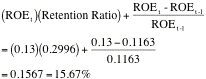
Expected Growth rate in EPS =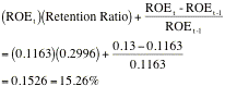

Growth in Operating Income

Just as equity income growth is determined by the equity reinvested back into the business and the return made on that equity investment, you can relate growth in operating income to total reinvestment made into the firm and the return earned on capital invested.

When a firm has a stable return on capital, its expected growth in operating income is a product of the reinvestment rate, i.e., the proportion of the after-tax operating income that is invested in net capital expenditures and non-cash working capital, and the quality of these reinvestments, measured as the return on the capital invested.

Expected Growth_EBIT = Reinvestment Rate * Return on Capital

where,

Return on Capital =

In making these estimates, you use the adjusted operating income and reinvestment values that you computed in Chapter 4. Both measures should be forward looking and the return on capital should represent the expected return on capital on future investments. In the rest of this section, you consider how best to estimate the reinvestment rate and the return on capital.

Reinvestment Rate

The reinvestment rate measures how much a firm is plowing back to generate future growth. The reinvestment rate is often measured using the most recent financial statements for the firm. Although this is a good place to start, it is not necessarily the best estimate of the future reinvestment rate. A firm’s reinvestment rate can ebb and flow, especially in firms that invest in relatively few, large projects or acquisitions. For these firms, looking at an average reinvestment rate over time may be a better measure of the future. In addition, as firms grow and mature, their reinvestment needs (and rates) tend to decrease. For firms that have expanded significantly over the last few years, the historical reinvestment rate is likely to be higher than the expected future reinvestment rate. For these firms, industry averages for reinvestment rates may provide a better indication of the future than using numbers from the past. Finally, it is important that you continue treating R&D expenses and operating lease expenses consistently. The R&D expenses, in particular, need to be categorized as part of capital expenditures for purposes of measuring the reinvestment rate.

Return on Capital

The return on capital is often based upon the firm's return on existing investments, where the book value of capital is assumed to measure the capital invested in these investments. Implicitly, you assume that the current accounting return on capital is a good measure of the true returns earned on existing investments and that this return is a good proxy for returns that will be made on future investments. This assumption, of course, is open to question for the following reasons.

· The book value of capital might not be a good measure of the capital invested in existing investments, since it reflects the historical cost of these assets and accounting decisions on depreciation. When the book value understates the capital invested, the return on capital will be overstated; when book value overstates the capital invested, the return on capital will be understated. This problem is exacerbated if the book value of capital is not adjusted to reflect the value of the research asset or the capital value of operating leases.

· The operating income, like the book value of capital, is an accounting measure of the earnings made by a firm during a period. All the problems in using unadjusted operating income described in Chapter 4 continue to apply.

· Even if the operating income and book value of capital are measured correctly, the return on capital on existing investments may not be equal to the marginal return on capital that the firm expects to make on new investments, especially as you go further into the future.

Given these concerns, you should consider not only a firm’s current return on capital, but any trends in this return as well as the industry average return on capital. If the current return on capital for a firm is significantly higher than the industry average, the forecasted return on capital should be set lower than the current return to reflect the erosion that is likely to occur as competition responds.

Finally, any firm that earns a return on capital greater than its cost of capital is earning an excess return. The excess returns are the result of a firm’s competitive advantages or barriers to entry into the industry. High excess returns locked in for very long periods imply that this firm has a permanent competitive advantage.

Illustration 11.9: Measuring the Reinvestment Rate, Return on Capital and Expected Growth Rate – Embraer and Amgen

In this Illustration, we will estimate the reinvestment rate, return on capital and expected growth rate for Embraer, the Brazilian aerospace firm, and Amgen. We begin by presenting the inputs for the return on capital computation in Table 11.8.

Table 11.8: Return on Capital

	EBIT	EBIT (1-t)	BV of Debt	BV of Equity	Return on Capital
Embraer	945	716.54	1321.00	697.00	35.51%
Amgen	$1,996	$1,500	$323	$5,933	23.98%

We use the effective tax rate for computing after-tax operating income and the book value of debt and equity from the end of the prior year. For Amgen, we use the operating income and book value of equity, adjusted for the capitalization of the research asset, as described in Illustration 9.2. The after-tax returns on capital are computed in the last column.

We follow up by estimating capital expenditures, depreciation and the change in non-cash working capital from the most recent year in Table 11.9.

Table 11.9: Reinvestment Rate

	EBIT(1-t)	Capital expenditures	Depreciation	Change in Working Capital	Reinvestment	Reinvestment Rate
Embraer	716.54	182.10	150.16	-173.00	-141.06	-19.69%
Amgen	$1,500.32	$1,283.00	$610.00	$121.00	$794.00	52.92%

Here again, we treat R&D as a capital expenditure and the amortization of the research asset as part of depreciation for computing the values for Amgen. In the last column, we compute the reinvestment rate by dividing the total reinvestment (cap ex – depreciation + Change in working capital) by the after-tax operating income. Note that Embraer’s reinvestment rate is negative because of non-cash working capital dropped by 173 million in the most recent year.

Finally, we compute the expected growth rate by multiplying the after-tax return on capital by the reinvestment rate in Table 11.10

Table 11.10: Expected Growth Rate in Operating Income

	Reinvestment Rate	Return on Capital	Expected Growth Rate
Embraer	-19.69%	35.51%	-6.99%
Amgen	52.92%	23.98%	12.69%

If Amgen can maintain the return on capital and reinvestment rate that they had last year, it would be able to grow at 12.69% a year. Embraer’s growth rate is negative because its reinvestment rate is negative. In the Illustration that follows, we will look at the reinvestment rate in more detail.

---

[1]