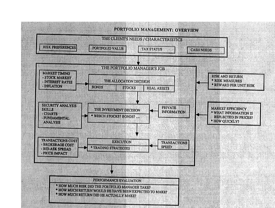
The trade off between Risk and Return

Most, if not all, investors are risk averse

To get them to take more risk, you have to offer higher expected returns

Conversely, if investors want higher expected returns, they have to be willing to take more risk.

Ways of evaluating risk

Most investors do not know have a quantitative measure of how much risk that they want to take

Traditional risk and return models tend to measure risk in terms of volatility or standard deviation

In the mean-variance world, variance is the only measure of risk. Investors given a choice between tow investments with the same expected returns but different variances, will always pick the one with the lower variance.

• In theoretical models, the expected returns and variances are in terms of future returns.
• In practice, the expected returns and variances are calculated using historical data and are used as proxies for future returns.

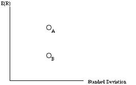
Illustration 1: Calculation of expected returns/standard deviation using historical returns

			GE						The Home Depot
Year	Price at		Dividends		Returns		Price at		Dividends		Returns
	end of year		during year				end of year		during year
1989	$ 32.25						$ 8.13
1990	$ 28.66		$ 0.95		-8.19%		$ 12.88		$ 0.04		58.82%
1991	$ 38.25		$ 1.00		36.95%		$ 33.66		$ 0.05		161.79%
1992	$ 42.75		$ 1.00		14.38%		$ 50.63		$ 0.07		50.60%
1993	$ 52.42		$ 1.00		24.96%		$ 39.50		$ 0.11		-21.75%
1994	$ 51.00		$ 1.00		-0.80%		$ 46.00		$ 0.15		16.84%
Average					13.46%						53.26%
Standard Deviation				18.42%						68.50%

Concept Check:

• While The Home Depot exhibited higher variance in returns, much of the variance seems to come from the stock price going up dramatically between 1989 and 1992? Why is this ìupsideî considered risk?
• Should risk not be defined purely in terms of "downside" potential (negative returns)?

mportfolio = w_A m_A + (1 - w_A) m_B

s²_portfolio = w_A² s²_A + (1 - w_A)² s²_B + 2 w_A w_B r_AB s_A s_B

where

w_A = Proportion of the portfolio in asset A

The last term in the variance formulation is sometimes written in terms of the covariance in returns between the two assets, which is

s_AB = r_AB s_A s_B

• The savings that accrue from diversification are a function of the correlation coefficient.

Illustration 2: Extending the two-asset case - GE and The Home Depot

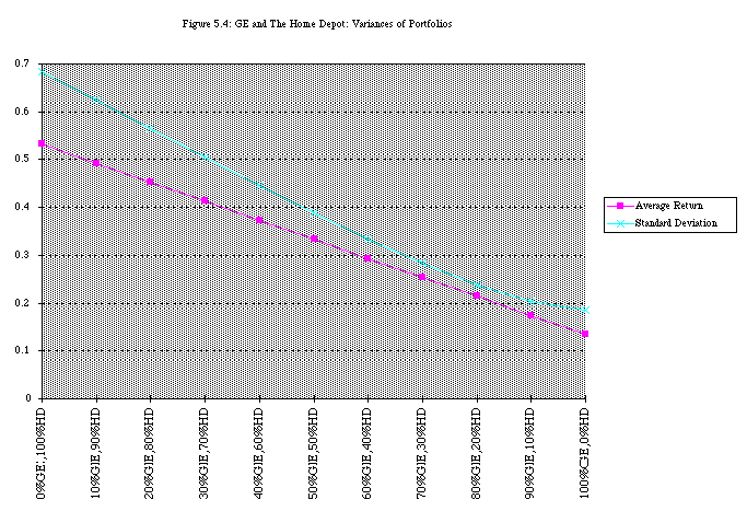
Step 1: Use historical data to estimate average returns and standard deviations in returns for the two investments.

Stock	Average Return (1990-94)	Standard Deviation (1990-94)
General Electric	13.46%	18.42%
The Home Depot	53.26%	68.50%

Step 2: Estimate the correlation and covariance in returns between the two investments using historical data.

Year	Returns on GE(RGe)	Returns on HD (RH)	(RGE- Avge(RGE))2	(RH-Avge(RH))2	(RGE- Avge(RGE) (RH-Avge(RH)
1990	-8.19%	58.82%	0.04686	0.00309	(0.01203)
1991	36.95%	161.79%	0.05518	1.17786	0.25494
1992	14.38%	50.60%	0.00008	0.00071	(0.00024)
1993	24.96%	-21.75%	0.01322	0.56265	(0.08625)
1994	-0.80%	16.84%	0.02034	0.13265	0.05194
Total			0.13568	1.87696	0.20835

Variance in GE Returns = 0.13568/4 = 0.0339 Standard Deviation in GE Returns = 0.0339^0.5 = 0.1842

Variance in HD Returns = 1.87696/4 = 0.4692 Standard Deviation in HD Returns = 0.4692^0.5 = 0.6850

Covariance between GE and The Home Depot Returns = 0.20835/4 = 0.0521

Correlation between GE and The Home Depot Returns =rGH = sGH /sG sH = 0.0521/(0.1842*0.6850) = 0.4129

Step 3: Compute the expected returns and variances of portfolios of the two securities using the statistical parameters estimates above ñ

Consider, for instance, a portfolio composed of 50% in GE and 50% in The Home Depot ñ

Average Return of Portfolio = 0.5 (13.46%) + 0.5 (53.26%) =

Variance of Portfolio = (0.5)2 (18.42%)2 + (0.5)2 (68.50%)2 + 2 (0.5) (0.5) (0.4129) (18.42%) (68.50%) = 1518%

Standard Deviation of Portfolio = 38.96%

From Two Assets To Three Assets to n Assets

The variance of a portfolio of three assets can be written as a function of the variances of each of the three assets, the portfolio weights on each and the correlations between pairs of the assets. The variance can be written as follows -

s_p²= w_A² s²_A + w_B² s²_B + w_C² s²_C+ 2 w_A w_B r_AB s_A s_B+ 2 w_A w_C r_AC s_A s_C+ 2 w_B w_C r_BC s_B s_C

where

w_A,w_B,w_C = Portfolio weights on assets

s²_A ,s²_B ,s²_C = Variances of assets A, B, and C

r_AB , r_AC , r_BC = Correlation in returns between pairs of assets (A&B, A&C, B&C)

where n is the number of assets in the portfolio

Number of Assets	Number of covariance terms
2	1
5	10
10	45
20	190
100	4950
1000	499500

Most Investors do not measure their risk preferences in terms of standard deviation

For other investors, risk has to be assessed by using

• Scoring Systems (where investors are asked for information or questions to answers which can be used to analyze how much risk an investor is willing to take)
• Risk categories (High; Average; Low)
• Life cycle theories of investing

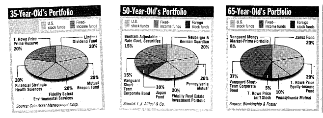
General Propositions:

As investors age, there will be a general increase in risk aversion, leading to greater allocation to safer asset classes.

• The value of a portfolio constrains your choices at later stages.
• This is because trading individual securities creates costs - brokerage costs, bid-ask spreads and price impact
• There is a critical mass value, below which it does not pay to actively manage a portfolio - it is far better to invest in funds.
• The larger a portfolio, the more choices become available in terms of assets - this is largely because some components of trading costs - the brokerate costs and the spread - may get smaller for larger portfolios.
• If a portfolio becomes too large, it might start creating a price impact which might cause trading costs to start increasing again.

	Stocks	Bonds
Market Returns	$ 534.46	$ 17.30
After Transactions Cost	$ 354.98	$ 11.47
After Income Taxes	$ 161.55	$ 4.91
After Capital Gains Taxes	$ 113.40	$ 4.87
After Inflation	$ 16.10	$ 0.69

Transactions Costs: 0.5% a year; Income taxes: at 28%; Capital Gains at 28% every 20 years;

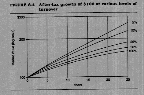
- What is a long time horizon?

- Determinants of time horizon

* Age

* Level of Income

* Stability of Income

* Cash Requirements

- Time Horizon and Asset Choice

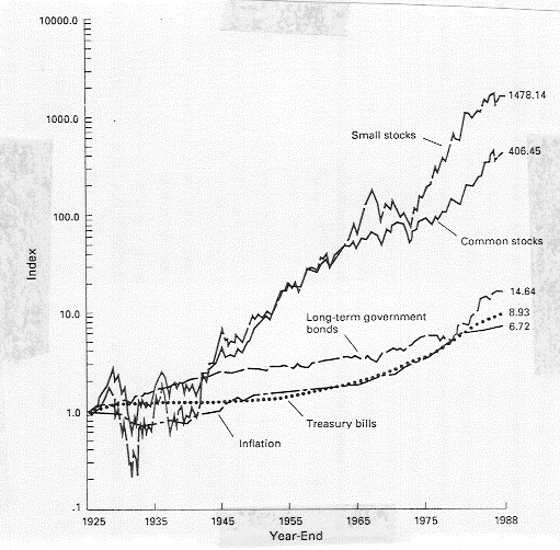
Proposition: The cost of keeping funds in near-cash investments increases with the time horizon of the investor.

• The first step in all portfolio management is the asset allocation decision.
• The asset allocation decision determines what proportions of the portfolio will be invested in different asset classes.
• Asset allocation can be passive,
  • It can be based upon the mean-variance framework
  • It can be based upon simpler rules of diversification or market value based
• When asset allocation is determined by market views, it is active asset allocation.

where,

s² = Investor's desired level of variance

E(R) = Investor's desired expected returns

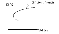
The portfolios that emerge from this process are called Markowitz portfolios. These portfolios are considered efficient, because they maximize expected returns given the standard deviation, and the entire set of portfolios is referred to as the Efficient Frontier. Graphically, these portfolios are shown on the expected return/standard deviation dimensions in figure 5.7 -

• If we have information on the expected returns and variances of different asset classes and the covariances between asset classes, we can devise efficient portfolios given any given level of risk.
• For example, if the following is the information of 4 asset classes:

Asset Class	Mean	Standard deviation
U.S. stocks	12.50%	16.50%
U.S. bonds	6.50%	5.00%
Foreign Stocks	15.00%	26.00%
Real Estate	11.00%	12.50%

	U.S. Stock	U.S. Bonds	Foreign Stocks	Real Estate
U.S. Stocks	1.00	0.65	0.35	0.25
U.S. Bonds		1.00	0.15	-0.10
Foreign Stocks			1.00	0.05
Real Estate				1.00

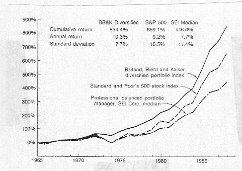
The objective is to create a portfolio to take advantage of 'forecasted' market movements, up or down. Strategies could include:

* Shifting from (to) overvalued asset classes to (from) undervalued asset classes if you expect the market to go up (down).

* Buying calls (puts) or buying (selling) futures on a market if you expect the market to go up (down).

Assumption: You can forecast market movements

Advantage: If you can forecast market movements, the rewards are immense.

Disadvantage: If you err, the costs can be significant.

Fairly unsophisticated strategies beat these funds..

• Once the asset allocation decision has been made, the portfolio manager has pick the securities that go into the portfolio.
• Again, the decision can be made on a passive basis or on active basis.
• Active security selection can take several forms:
  • it can be based upon fundamentals
  • it can be based upon technical indicators
  • it can be based upon ìinformationî

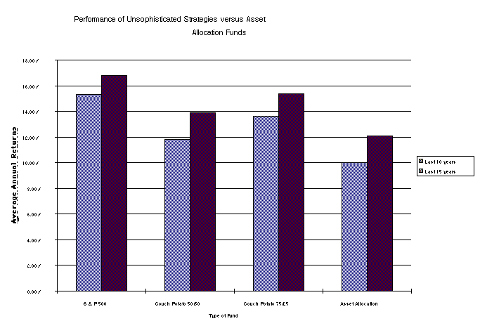
Index funds are created by holding stocks in a wider index in proportion to their market value. No attempt is made to trade on a frequent basis to catch market upswings or downswings or select 'good' stocks.

Assumptions: Markets are efficient. Attempts to time the market and pick good stocks are expensive and do not provide reasonable returns. Holding a well diversified portfolio eliminates unsystematic risk.

Advantages: Transactions costs are minimal as is the cost of searching for information.

B. Markowitz Portfolio: A Markowitz efficient portfolio is created by searching through all possible combinations of the universe of securities to find that combination that maximizes expected return for any given level of risk.

Assumptions: The portfolio manager can identify the inputs (mean, variance, covariance) to the model correctly and has enough computer capacity to run through the optimization exercise.

Advantages: If historical data is used, the process is inexpensive and easily mechanised.

Disadvantages: The model is only as good as its inputs.

The objective is to use the skills of your security analysts to select stocks that will outperform the market, and create a portfolio of these stocks. The security selection skills can take on several forms.

(1) Technical Analysis, where charts reveal the direction of future price movements

(2) Fundamental Analysis, where public information is used to pick undervalued stocks

(3) Access to private information, which enables the analyst to pinpoint mis-valued securities.

Assumption: Your stock selection skills help you make choices which, on average, beat the market.

Inputs: The model will vary with the security selection model used.

Advantage: If there are systematic errors in market valuation andyour model can spot these errors, the portfolio will outperform others in the market.

Disadvantage: If your security selection does not pay off, you have expended time and resources to earn what another investor could have made with random selection.Security Selection strategies vary widely and can lead to contradictory recommendations..

• Technical investors can be
  • momentum investors, who buy on strength and sell on weakness
  • reversal investors, who do the exact opposite
• Fundamental investors can be
  • value investors, who buy low PE orlow PBV stocks which trade at less than the value of assets in place
  • growth investors, who buy high PE and high PBV stocks which trade at less than the value of future growth
• Information traders can believe
  • that markets learn slowly and buy on good news and sell on bad news
  • that markets overreact and do the exact opposite

• The cost of trading includes the brokerage cost, the bid-ask spread and the price impact

• There are two components to trading and execution - the cost of execution (trading) and the speed of execution.
• Generally speaking, the tradeoff is between faster execution and lower costs.
• For some active strategies (especially those based on information) speed is of the essence.

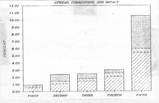
Maximize: Speed of Execution

Subject to: Cost of execution < Excess returns from strategy

• For other active strategies (such as long term value investing) the cost might be of the essence.

Minimize: Cost of Execution

Subject to: Speed of execution < Specified time period.

• The larger the fund, the more significant this trading cost/speed tradeoff becomes.

* Who should measure performance?

Performance measurement has to be done either by the client or by an objective third party on the basis of agreed upon criteria. It should not be done by the portfolio manager.

* How often should performance be measured?

The frequency of portfolio evaluation should be a function of both the time horizon of the client and the investment philosophy of the portfolio manager. However, portfolio measurement and reporting of value to clients should be done on a frequent basis.

* How should performance be measured?

I. Market Indices (No adjustment for risk): There are some who do not like models for risk and return and prefer comparison to broad market indices (S&P 500, NYSE composite, ..)

The limitation of this approach is that it does not explicitly control for risk. Thus, an advantage is given to risky funds and money managers.

Tracking Error as a Measure of Risk

Tracking error measures the difference between a portfolioís return and its benchmark index. Thus portfolios that deliver higher returns than the benchmark

II. Against other portfolio managers

In some cases, portfolio managers are measured against other portfolio managers who have similar objective functions. Thus, a growth fund manager may be measured against all growth fund managers.

III. Risk-Adjusted Models

A. The CAPM: The capital asset pricing model provides a simple and intuitive measure for measuring performance. It compares the actual returns made by a portfolio manager with the returns he should have made, given both market performance during the period and the beta of the portfolio created by the manager.

Abnormal Return = Actual Return - Expected Return

> 0: Outperformed

< 0: Underperformed

where,

Actual Return = Returns on the portfolio (including dividends)

Expected Return = Riskfree rate at the start of the period + Beta of portfolio * (Actual return on market during the period - Riskfree Rate)

This abnormal return is called Jensen's Alpha. It can also be computed by regressing the returns on the portfolio against a market index, and then comparing the intercept to Rf (1- Beta).

Variants: Define Rp to be the return on the portfolio and Rm to be the return on the market.

Treynor Index = (Rp - Rf)/ Beta of the portfolio

> (Rm - Rf) : Outperformed

< (Rm - Rf) : Underperformed

Sharpe Index = (Rp - Rf)/ Variance of the portfolio

> (Rm - Rf)/sm : Outperformed

< (Rm - Rf)/sm : Underperformed

Information Ratio = Jensenís alpha / Unsystematic Risk

> 0: Outperformed the market

< 0 : Underperformed

• Tracking error measures the difference between a portfolioís return and its benchmark index. Thus portfolios that deliver higher returns than the benchmark but have higher tracking error are considered riskier.
• Tracking error is a way of ensuring that a portfolio stays within the same risk level as the benchmark index.
• It is also a way in which the ìactiveî in active money management can be constrained.

Performance Attribtion

This analysis can be carried one step forward, and the overall performance of a money manager can be decomposed into ìmarket timingî and ìsecurity selectionî components.

• If money managers are good market timers,
  • they should hold high beta stocks, when the the return on the market > risk free rate
  • they should hold low beta stocks, when the return on the market < risk free rate
• Thus, the market timing capabilities of a money manager can be evaluated by looking at the managerís performance over time relative to the market. For instance, consider the following funds ñ

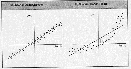
In some cases, better estimates of market timing can be obtained by fitting a quadratic curve to actual returns.

where c is a measure of the market timing ability of a fund (money manager).

B. The APT: The arbitrage pricing theory defines the expected return in terms of statistical factors (instead of just the market as in the CAPM). A beta is defined relative to each factor.

C. Multi-Index Models: Multi-index models allow the performance evaluator to bring in economic factors that may influence expected returns.

* Window Dressing and other Phenomena that cloud measurement

1. Marking up the merchandise (thinly traded stocks)

2. Tricking the technicians (stocks with breakout points)

3. Playing catch up (Buying hot stocks just before evaluation)

4. Dumping the losers just before evaluation