APPLICATIONS OF OPTION PRICING THEORY TO EQUITY VALUATION
Application of option pricing models to valuation
A few caveats on applying option pricing models
1. The underlying asset is not traded
2. The price of the asset follows a continuous process
3. The variance is known and does not change over the life of the option
4. Exercise is instantaneous
I. Valuing Equity as an option
The General Framework
Equity as a call option
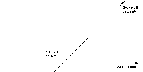
Payoff to equity on liquidation
= V - D if V > D
= 0 if V
where,
V = Value of the firm
D = Face Value of the outstanding debt and other external claims
Payoff on exercise = S - K if S > K
= 0 if S
Payoff Diagram for Equity as a Call Option

Illustration 3: Application to valuation: A simple example
Model Parameters
The parameters of equity as a call option are as follows:
Value of the underlying asset = S = Value of the firm = $ 100
million
Exercise price = K = Face Value of outstanding debt = $ 80 million
Life of the option = t = Life of zero-coupon debt = 10 years
Variance in the value of the underlying asset = s2 = Variance in firm value = 0.16
Riskless rate = r = Treasury bond rate corresponding to option
life = 10%
Valuing Equity as a Call Option
Based upon these inputs, the Black-Scholes model provides the
following value for the call:
d1 = 1.5994 N(d1) = 0.9451
d2 = 0.3345 N(d2) = 0.6310
Value of the call = 100 (0.9451) - 80 exp(-0.10)(10) (0.6310)
= $75.94 million
Value of the outstanding debt = $100 - $75.94 = $24.06 million
Interest rate on debt = ($ 80 / $24.06)1/10 -1 = 12.77%
Implications of viewing equity as a call option
A. Valuing equity in a troubled firm
Illustration 4 : Value of a troubled firm
The parameters of equity as a call option are as follows:
Value of the underlying asset = S = Value of the firm = $ 50 million
Exercise price = K = Face Value of outstanding debt = $ 80 million
Life of the option = t = Life of zero-coupon debt = 10 years
Variance in the value of the underlying asset = s2 = Variance in firm value = 0.16
Riskless rate = r = Treasury bond rate corresponding to option
life = 10%
Valuing Equity in a Troubled Firm
Based upon these inputs, the Black-Scholes model provides the
following value for the call:
d1 = 1.0515 N(d1) = 0.8534
d2 = -0.2135 N(d2) = 0.4155
B. The Conflict between bondholders and stockholders
Illustration 5: Effect on value of the conflict between stockholders and bondholders
Value of Equity = $75.94 million
Value of Debt = $24.06 million
Value of Firm == $100 million
Valuing Equity after the Project
Value of the underlying asset = S = Value of the firm = $ 100
million - $2 million = $ 98 million (The value of the firm is
lowered because of the negative net present value project)
Exercise price = K = Face Value of outstanding debt = $ 80 million
Life of the option = t = Life of zero-coupon debt = 10 years
Variance in the value of the underlying asset = s2 = Variance in firm value = 0.25
Riskless rate = r = Treasury bond rate corresponding to option
life = 10%
Based upon these inputs, the Black-Scholes model provides the
following value for the equity and debt in this firm.
Value of Equity = $77.71
Value of Debt = $20.29
Value of Firm = $98.00
Illustration 6: Effects on equity of a conglomerate merger
You are provided information on two firms, which operate in unrelated
businesses and hope to merge.
Firm A Firm B
Value of the firm $100 million $ 150 million
Face Value of Debt $ 80 million $ 50 million (Zero-coupon debt)
Maturity of debt 10 years 10 years
Std. Dev. in firm value 40 % 50 %
Correlation between firm
cashflows 0.4
The ten-year bond rate is 10%.
Variance in combined firm value = w12 s12 + w22 s22 + 2 w1 w2 r12 s1 s2
= (0.4)2 (0.16) + (0.6)2 (0.25) + 2 (0.4) (0.6) (0.4) (0.4) (0.5)
= 0.154
Valuing the Combined Firm
The values of equity and debt in the individual firms and the
combined firm can then be estimated using the option pricing model:
Firm A Firm B Combined firm
Value of equity in the firm $75.94 $134.47 $ 207.43
Value of debt in the firm $24.06 $ 15.53 $ 42.57
Value of the firm $100.00 $150.00 $ 250.00
Obtaining option pricing inputs - Some real world problems
The examples that have been used to illustrate the use of option
pricing theory to value equity have made some simplifying assumptions.
Among them are the following:
(1) There were only two claim holders in the firm - debt and equity.
(2) There is only one issue of debt outstanding and it can be
retired at face value.
(3) The debt has a zero coupon and no special features (convertibility,
put clauses etc.)
(4) The value of the firm and the variance in that value can be
estimated.
Applicability in valuation
|
|
|
| Value of the Firm |
|
| Variance in Firm Value |
s2firm = we2 se2 + wd2 sd2 + 2 we wd red sesd
|
| Maturity of the Debt |
|
North America $ 400 million
Europe $ 500 million
South America $ 100 million
Maturity Face Value Coupon Duration
20 year debt $ 100 mil 11% 14.1 years
15 year debt $ 100 mil 12% 10.2 years
10 year debt $ 200 mil 12% 7.5 years
1 year debt $ 800 mil 12.5% 1 year
Valuing Equity in the Airline
Step 1: Estimate the value of the firm = Sum of the value of its
assets = 400 + 500 + 100 = 1,000 million
Step 2: Estimate the average duration of the debt outstanding
= (100/1200) * 14.1 + (100/1200) * 10.2 + (200/1200) * 7.5 + (800/1200)
* 1 = 3.9417 years
Step 3: Estimate the face value of debt outstanding = 100 + 100
+ 200 + 800 = 1,200 million
Step 4: Estimate the variance in the value of the firm = Weighted
average of the variances in stock and bond prices. =
Variance of the firm = (E/(D+E))2 se2 + (D/(D+E))2 sd2 + 2 (E/(D+E)) (D/(D+E)) red sesd
= (.1)2 (.25)2 + (.9)2 (.10)2 + 2 (.1)(.9)(.3) (.25)(.10) = 0.010075
Step 5: Value equity as an option
d1 = 0.7671 N(d1) = 0.7784
d2 = 0.5678 N(d2) = 0.7148
Value of the call = 1000 (0.7784) - 1200 exp(-0.08)(3.9417) (0.7148) = $ 152.63 million
Debt Type Face Value Duration
Short term Debt $ 865 mil 0.5 years
Bank Debt $ 480 mil 3.0 years
Senior Debt $ 832 mil 6.0 years
Senior Subordinated $ 823 mil 8.5 years
Total $ 3000 mil 4.62 years
Cost of Capital in high growth period = 16.03% (0.2986) + 10%
(1 - 0.36) (0.7014) = 9.27%
Cost of Capital in terminal period = 13.55% (0.50) + 8.50% (1
- 0.36) (0.50) = 9.34%
|
|
|
|
|
|
|
|
|
|
|
|
|
| Revenues |
|
|
|
|
|
|
|
|
|
|
|
| - COGS |
|
|
|
|
|
|
|
|
|
|
|
| - Depreciation |
|
|
|
|
|
|
|
|
|
|
|
| EBIT |
|
|
|
|
|
|
|
|
|
|
|
| - EBIT*t |
|
|
|
|
|
|
|
|
|
|
|
| EBIT (1-t) |
|
|
|
|
|
|
|
|
|
|
|
| + Depreciation |
|
|
|
|
|
|
|
|
|
|
|
| -Capital Spending |
|
|
|
|
|
|
|
|
|
|
|
| - Æ Wking Capital |
|
|
|
|
|
|
|
|
|
|
|
| Free CF to Firm |
|
|
|
|
|
|
|
|
|
|
|
The stock and bond price variance are first annualized:
Annualized variance in stock price = 0.0133 * 12 = 0.16 Standard
deviation = 0.40
Annualized variance in bond price = 0.0012 * 12 = 0.0144 Standard
deviation = 0.12
Annualized variance in firm value
= (0.30)2 (0.16) + (0.70)2 (0.0.0144) + 2 (0.3) (0.7)(0.25)(0.40)(0.12)=
0.02637668
The parameters of equity as a call option are as follows:
Value of the underlying asset = S = Value of the firm = $ 2871
million
Exercise price = K = Face Value of outstanding debt = $ 3000 million
Life of the option = t = Weighted average duration of debt = 4.62
years
Variance in the value of the underlying asset = s2 = Variance in firm value = 0.0264
Riskless rate = r = Treasury bond rate corresponding to option
life = 7%
Based upon these inputs, the Black-Scholes model provides the
following value for the call:
d1 = 0.9910 N(d1) = 0.8391
d2 = 0.6419 N(d2) = 0.7391
Value of the call = 2871 (0.8391) - 3000 exp(-0.07)(4.62) (0.7395) = $ 817 million
Cablevision's equity was trading at $1100 million in March 1995.
II. Valuing Natural Resource Options/ Firms
The General Framework
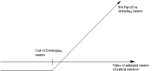
Payoff on natural resource investment = V - X if V > X
= 0 if V
Payoff on a Natural Resource Investment

Obtaining the inputs for valuing natural resource options
|
|
|
| 1. Value of Available Reserves of the Resource |
|
| 2. Cost of Developing Reserve (Strike Price) |
|
| 3. Time to Expiration |
|
| 4. Variance in value of underlying asset |
|
| 5. Net Production Revenue (Dividend Yield) |
|
| 6. Development Lag |
|
Inputs for the Option Pricing Model
Value of the underlying asset = Present Value of expected gold
sales (@ 50,000 ounces a year) = (50,000 * 350) * (1- (1.0320/1.1020))/(.10-.03)
- (50,000*250)* (1- (1.0420/1.1020))/(.10-.04) = $ 42.40 million
Exercise price = PV of Cost of opening mine = $40 million
Variance in ln(gold price) = 0.04
Time to expiration on the option = 20 years
Riskless interest rate = 9%
Dividend Yield = Loss in production for each year of delay = 1
/ 20 = 5%
(Note: It will take twenty years to empty the mine, and the firm
owns the rights for twenty years. Every year of delay implies
a loss of one year of production.)
Valuing the Option
Based upon these inputs, the Black-Scholes model provides the
following value for the call:
d1 = 1.4069 N(d1) = 0.9202
d2 = 0.5124 N(d2) = 0.6958
Call Value= 42.40 exp(-0.05)(20) (0.9202) -40 (exp(-0.09)(20)
(0.6958)= $ 9.75 million
The value of the mine as an option is $ 9.75 million, in contrast
to the static capital budgeting analysis which would have yielded
a net present value of $ 2.40 million ($42.40 million - $ 40 million).
The additional value accrues directly from the mine's option characteristics.
Illustration 10: Valuing an oil reserve
Inputs to the Black-Scholes Model
Given this information, the inputs to the Black-Scholes can be
estimated as follows:
Current Value of the asset = S = Value of the developed reserve
discounted back the length of the development lag at the dividend
yield = $12 * 50 /(1.05)2 = $ 544.22
(If development is started today, the oil will not be available
for sale until two years from now. The estimated opportunity cost
of this delay is the lost production revenue over the delay period.
Hence, the discounting of the reserve back at the dividend yield)
Exercise Price = Present Value of development cost = $12 * 50
= $600 million
Time to expiration on the option = 20 years
Variance in the value of the underlying asset = 0.03
Riskless rate =8%
Dividend Yield = Net production revenue / Value of reserve = 5%
Valuing the Option
Based upon these inputs, the Black-Scholes model provides the
following value for the call:
d1 = 1.0359 N(d1) = 0.8498
d2 = 0.2613 N(d2) = 0.6030
Call Value= 544 .22 exp(-0.05)(20) (0.8498) -600 (exp(-0.08)(20)
(0.6030)= $ 97.08 million
This oil reserve, though not viable at current prices, still is
a valuable property because of its potential to create value if
oil prices go up.
Extending the option pricing approach to value natural resource
firms
Inputs to the Black-Scholes Model
Input to model Corresponding input for valuing natural resource
firm
Value of underlying asset Value of cumulated estimated reserves
of the resource owned by the firm, discounted back at the dividend
yield for the development lag.
Exercise Price Estimated cumulated cost of developing estimated
reserves
Time to expiration on option Average relinquishment period across
all reserves owned by firm (if known) or estimate of when reserves
will be exhausted, given current production rates.
Riskless rate Riskless rate corresponding to life of the option
Variance in value of asset Variance in the price of the natural
resource
Dividend yield Estimated annual net production revenue as percentage
of value of the reserve.
Illustration 11: Valuing an oil company - Gulf Oil in 1984
Valuing the Option
Value of underlying asset = Value of estimated reserves discounted
back for period of development lag= 3038 * ($ 22.38 - $7) / 1.052
= $42,380.44
Exercise price = Estimated development cost of reserves = 3038
* $10 = $30,380 million
Time to expiration = Average length of relinquishment option =
12 years
Variance in value of asset = Variance in oil prices = 0.03
Riskless interest rate = 9%
Dividend yield = Net production revenue/ Value of developed reserves
= 5%
Based upon these inputs, the Black-Scholes model provides the
following value for the call:
d1 = 1.6548 N(d1) = 0.9510
d2 = 1.0548 N(d2) = 0.8542
Call Value= 42,380.44 exp(-0.05)(12) (0.9510) -30,380 (exp(-0.09)(12)
(0.8542)= $ 13,306 million
Valuing Gulf Oil
Value of already developed reserves = 915 (1 - 1.125-10)/.125
= $5065.83
Adding the value of the developed and undeveloped reserves of
Gulf Oil provides the value of the firm.
Value of undeveloped reserves = $ 13,306 million
Value of production in place = $ 5,066 million
Total value of firm = $ 18,372 million
Less Outstanding Debt = $ 9,900 million
Value of Equity = $ 8,472 million
Value per share = $ 8,472/165.3 = $51.25
This analysis would suggest that Gulf Oil was overvalued at $70
per share.
III. Valuing product patents as options
The General Framework
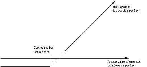
Payoff from owning a product patent = V - I if V> I
= 0 if V

Obtaining the inputs for option valuation
|
|
|
| 1. Value of the Underlying Asset |
|
| 2. Variance in value of underlying asset |
|
| 3. Exercise Price on Option |
|
| 4. Expiration of the Option |
|
| 5. Dividend Yield |
|
Valuing the Option
The inputs to the option pricing model are as follows:
Value of the underlying asset = Present value of inflows (current)
= $1,000 million
Exercise price = Present value of cost of developing product =
$1,500 million
Time to expiration = Life of the patent = 20 years
Variance in value of underlying asset = Variance in PV of inflows
= 0.03
Riskless rate = 10%
Based upon these inputs, the Black-Scholes model provides the
following value for the call:
d1 = 1.1548 N(d1) = 0.8759
d2 = 0.3802 N(d2) = 0.6481
Call Value= 1000 exp(-0.05)(20) (0.8759) -1500 (exp(-0.10)(20)
(0.6481)= $ 190.66 million
Illustration 13: Valuing a firm with only product options
Inputs to the Option Pricing Model
The inputs to the option pricing model are as follows:
Value of underlying asset = Present value of expected cashflows
= $ 500 million
Exercise price = Present value of cost of developing product for
commercial use = $400 mil
Time to expiration on the option = Time to expiration on patent
rights = 25 years
Variance in value of underlying asset = 0.20
Riskless rate = 7%
Dividend yield = Expected annual cashflow / PV of cash inflows
= 4%
Based upon these inputs, the Black-Scholes model provides the
following value for the call:
d1 = 1.5532 N(d1) = 0.9398
d2 = -0.6828 N(d2) = 0.2474
Call Value= 500 exp(-0.04)(25) (0.9398) - 400 (exp(-0.07)(25)
(0.2474)= $ 155.66 million
Valuing Biogen
Value of Existing Products = $ 12.14
Present Value of Cash Flows from Introducing the Drug Now = S
= $ 3.422 billion
Present Value of Cost of Developing Drug for Commercial Use =
K = $ 2.875 billion
Patent Life = t = 17 years Riskless Rate = r = 6.7% (17-year T.Bond
rate)
Variance in Expected Present Values =s2 = 0.224 (Industry average firm variance for bio-tech firms)
Expected Cost of Delay = y = 1/17 = 5.89%
d1 = 1.1362 N(d1) = 0.8720
d2 = -0.8512 N(d2) = 0.2076
Call Value= 3,422 exp(-0.0589)(17) (0.8720) - 2,875 (exp(-0.067)(17) (0.2076)= $ 907 million
Call Value per Share from Avonex = $ 907 million/35.5 million
= $ 25.55
Biogen Value Per Share = Value of Existing Assets + Value of Patent
= $ 12.14 + $ 25.55 = $ 37.69