The Little Book of Valuation

Intrinsic valuation

In intrinsic valuation, the value of an asset is estimated based upon its cash flows, growth potential and risk. In its most common form, we use the discounted cash flow approach to estimate intrinsic value, and the present value of the expected cashflows on the asset, discounted back at a rate that reflects the riskiness of these cashflows. In discounted cash flow valuation, we begin with a simple proposition. The value of an asset is not what someone perceives it to be worth but it is a function of the expected cash flows on that asset. Put simply, assets with high and predictable cash flows should have higher values than assets with low and volatile cash flows. In discounted cash flow valuation, we estimate the value of an asset as the present value of the expected cash flows on it.

where,

n = Life of the asset

E(CFt) = Expected cashflow in period t

r = Discount rate reflecting the riskiness of the estimated cashflows

The cashflows will vary from asset to asset -- dividends for stocks, coupons (interest) and the face value for bonds and after-tax cashflows for a business. The discount rate will be a function of the riskiness of the estimated cashflows, with higher rates for riskier assets and lower rates for safer ones.

Using discounted cash flow models is in some sense an act of faith. We believe that every asset has an intrinsic value and we try to estimate that intrinsic value by looking at an asset’s fundamentals. What is intrinsic value? Consider it the value that would be attached to an asset by an all-knowing analyst with access to all information available right now and a perfect valuation model. No such analyst exists, of course, but we all aspire to be as close as we can to this perfect analyst. The problem lies in the fact that none of us ever gets to see what the true intrinsic value of an asset is and we therefore have no way of knowing whether our discounted cash flow valuations are close to the mark or not.

There are three distinct ways in which we can categorize discounted cash flow models. In the first, we differentiate between valuing a business as a going concern as opposed to a collection of assets. In the second, we draw a distinction between valuing the equity in a business and valuing the business itself. In the third, we lay out three different and equivalent ways of doing discounted cash flow valuation – the expected cash flow approach, a value based upon excess returns and adjusted present value.

a. Going Concern versus Asset Valuation

The value of an asset in the discounted cash flow framework is the present value of the expected cash flows on that asset. Extending this proposition to valuing a business, it can be argued that the value of a business is the sum of the values of the individual assets owned by the business. While this may be technically right, there is a key difference between valuing a collection of assets and a business. A business or a company is an on-going entity with assets that it already owns and assets it expects to invest in the future. This can be best seen when we look at the financial balance sheet (as opposed to an accounting balance sheet) for an ongoing company in figure 1.1:

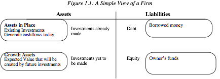
Note that investments that have already been made are categorized as assets in place, but investments that we expect the business to make in the future are growth assets.

A financial balance sheet provides a good framework to draw out the differences between valuing a business as a going concern and valuing it as a collection of assets. In a going concern valuation, we have to make our best judgments not only on existing investments but also on expected future investments and their profitability. While this may seem to be foolhardy, a large proportion of the market value of growth companies comes from their growth assets. In an asset-based valuation, we focus primarily on the assets in place and estimate the value of each asset separately. Adding the asset values together yields the value of the business. For companies with lucrative growth opportunities, asset-based valuations will yield lower values than going concern valuations.

One special case of asset-based valuation is liquidation valuation, where we value assets based upon the presumption that they have to be sold now. In theory, this should be equal to the value obtained from discounted cash flow valuations of individual assets but the urgency associated with liquidating assets quickly may result in a discount on the value. How large the discount will be will depend upon the number of potential buyers for the assets, the asset characteristics and the state of the economy.

b. Equity Valuation versus Firm Valuation

There are two ways in which we can approach discounted cash flow valuation. The first is to value the entire business, with both assets-in-place and growth assets; this is often termed firm or enterprise valuation.

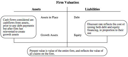
The cash flows before debt payments and after reinvestment needs are called free cash flows to the firm, and the discount rate that reflects the composite cost of financing from all sources of capital is called the cost of capital.

The second way is to just value the equity stake in the business, and this is called equity valuation.

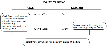
The cash flows after debt payments and reinvestment needs are called free cash flows to equity, and the discount rate that reflects just the cost of equity financing is the cost of equity.

Note also that we can always get from the former (firm value) to the latter (equity value) by netting out the value of all non-equity claims from firm value. Done right, the value of equity should be the same whether it is valued directly (by discounting cash flows to equity a the cost of equity) or indirectly (by valuing the firm and subtracting out the value of all non-equity claims). We will return to discuss this proposition in far more detail in a later chapter.

c. Variations on DCF Models

The model that we have presented in this section, where expected cash flows are discounted back at a risk-adjusted discount rate, is the most commonly used discounted cash flow approach but there are two widely used variants. In the first, we separate the cash flows into excess return cash flows and normal return cash flows. Earning the risk-adjusted required return (cost of capital or equity) is considered a normal return cash flow but any cash flows above or below this number are categorized as excess returns; excess returns can therefore be either positive or negative. With the excess return valuation framework, the value of a business can be written as the sum of two components:

Value of business = Capital Invested in firm today + Present value of excess return cash flows from both existing and future projects

If we make the assumption that the accounting measure of capital invested (book value of capital) is a good measure of capital invested in assets today, this approach implies that firms that earn positive excess return cash flows will trade at market values higher than their book values and that the reverse will be true for firms that earn negative excess return cash flows.

In the second variation, called the adjusted present value (APV) approach, we separate the effects on value of debt financing from the value of the assets of a business. In general, using debt to fund a firm’s operations creates tax benefits (because interest expenses are tax deductible) on the plus side and increases bankruptcy risk (and expected bankruptcy costs) on the minus side. In the APV approach, the value of a firm can be written as follows:

Value of business = Value of business with 100% equity financing + Present value of Expected Tax Benefits of Debt – Expected Bankruptcy Costs

In contrast to the conventional approach, where the effects of debt financing are captured in the discount rate, the APV approach attempts to estimate the expected dollar value of debt benefits and costs separately from the value of the operating assets.

While proponents of each approach like to claim that their approach is the best and most precise, we will show later in the book that the three approaches yield the same estimates of value, if we make consistent assumptions.

Relative Valuation

While the focus in classrooms and academic discussions remains on discounted cash flow valuation, the reality is that most assets are valued on a relative basis. In relative valuation, we value an asset by looking at how the market prices similar assets. Thus, when determining what to pay for a house, we look at what similar houses in the neighborhood sold for rather than doing an intrinsic valuation. Extending this analogy to stocks, investors often decide whether a stock is cheap or expensive by comparing its pricing to that of similar stocks (usually in its peer group). In this section, we will consider the basis for relative valuation, ways in which it can be used and its advantages and disadvantages.

In relative valuation, the value of an asset is derived from the pricing of 'comparable' assets, standardized using a common variable. Included in this description are two key components of relative valuation. The first is the notion of comparable or similar assets. From a valuation standpoint, this would imply assets with similar cash flows, risk and growth potential. In practice, it is usually taken to mean other companies that are in the same business as the company being valued. The other is a standardized price. After all, the price per share of a company is in some sense arbitrary since it is a function of the number of shares outstanding; a two for one stock split would halve the price. Dividing the price or market value by some measure that is related to that value will yield a standardized price. When valuing stocks, this essentially translates into using multiples where we divide the market value by earnings, book value or revenues to arrive at an estimate of standardized value. We can then compare these numbers across companies.

The simplest and most direct applications of relative valuations are with real assets where it is easy to find similar assets or even identical ones. The asking price for a Mickey Mantle rookie baseball card or a 1965 Ford Mustang is relatively easy to estimate given that there are other Mickey Mantle cards and 1965 Ford Mustangs out there and that the prices at which they have been bought and sold can be obtained. With equity valuation, relative valuation becomes more complicated by two realities. The first is the absence of similar assets, requiring us to stretch the definition of comparable to include companies that are different from the one that we are valuing. After all, what company in the world is remotely similar to Microsoft or GE? The other is that different ways of standardizing prices (different multiples) can yield different values for the same company.

Harking back to our earlier discussion of discounted cash flow valuation, we argued that discounted cash flow valuation was a search (albeit unfulfilled) for intrinsic value. In relative valuation, we have given up on estimating intrinsic value and essentially put our trust in markets getting it right, at least on average.

In relative valuation, the value of an asset is based upon how similar assets are priced. In practice, there are three variations on relative valuation, with the differences primarily in how we define comparable firms and control for differences across firms:

a. Direct comparison: In this approach, analysts try to find one or two companies that look almost exactly like the company they are trying to value and estimate the value based upon how these “similar” companies are priced. The key part in this analysis is identifying these similar companies and getting their market values.

b. Peer Group Average: In the second, analysts compare how their company is priced (using a multiple) with how the peer group is priced (using the average for that multiple). Thus, a stock is considered cheap if it trade at 12 times earnings and the average price earnings ratio for the sector is 15. Implicit in this approach is the assumption that while companies may vary widely across a sector, the average for the sector is representative for a typical company.

c. Peer group average adjusted for differences: Recognizing that there can be wide differences between the company being valued and other companies in the comparable firm group, analysts sometimes try to control for differences between companies. In many cases, the control is subjective: a company with higher expected growth than the industry will trade at a higher multiple of earnings than the industry average but how much higher is left unspecified. In a few cases, analysts explicitly try to control for differences between companies by either adjusting the multiple being used or by using statistical techniques. As an example of the former, consider PEG ratios. These ratios are computed by dividing PE ratios by expected growth rates, thus controlling (at least in theory) for differences in growth and allowing analysts to compare companies with different growth rates. For statistical controls, we can use a multiple regression where we can regress the multiple that we are using against the fundamentals that we believe cause that multiple to vary across companies. The resulting regression can be used to estimate the value of an individual company. In fact, we will argue later in this book that statistical techniques are powerful enough to allow us to expand the comparable firm sample to include the entire market.