 The
Little Book of Valuation
The
Little Book of Valuation
Summarizing Data
Large amounts of
data are often compressed into more easily assimilated summaries, which provide
the user with a sense of the content, without overwhelming him or her with too
many numbers. There a number of ways data can be presented. We will consider
two here—one is to present the data in a distribution, and the other is
to provide summary statistics that capture key aspects of the data.
Data Distributions
When presented
with thousands of pieces of information, you can break the numbers down into
individual values (or ranges of values) and indicate the number of individual
data items that take on each value or range of values. This is called a frequency distribution. If the data can only take on specific values, as is
the case when we record the number of goals scored in a soccer game, you get a discrete distribution. When the data can take on any value within the range,
as is the case with income or market capitalization, it is called a continuous distribution.
The advantages of
presenting the data in a distribution are twofold. For one thing, you can
summarize even the largest data sets into one distribution and get a measure of
what values occur most frequently and the range of high and low values. The
second is that the distribution can resemble one of the many common ones about
which we know a great deal in statistics. Consider, for instance, the
distribution that we tend to draw on the most in analysis: the normal
distribution, illustrated in Figure A1.1.
 A
normal distribution is symmetric, has a peak centered around the middle of the
distribution, and tails that are not fat and stretch to include infinite positive
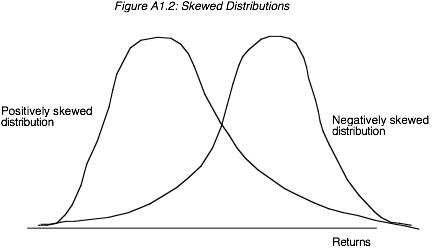
or negative values. Not all
distributions are symmetric, though. Some are weighted towards extreme positive
values and are called positively skewed, and some towards extreme negative
values and are considered negatively skewed. Figure A1.2 illustrates positively
and negatively skewed distributions.
A
normal distribution is symmetric, has a peak centered around the middle of the
distribution, and tails that are not fat and stretch to include infinite positive
or negative values. Not all
distributions are symmetric, though. Some are weighted towards extreme positive
values and are called positively skewed, and some towards extreme negative
values and are considered negatively skewed. Figure A1.2 illustrates positively
and negatively skewed distributions.
Summary Statistics
The simplest way
to measure the key characteristics of a data set is to estimate the summary
statistics for the data. For a data series, X1, X2, X3,
. . . Xn,
where n is the number of observations
in the series, the most widely used summary statistics are as follows:
• The mean (m), which
is the average of all of the observations in the data series.

• The median, which is the midpoint of the series; half the data
in the series is higher than the median and half is lower.
• The
variance, which is a measure of the spread in the distribution around the mean
and is calculated by first summing up the squared deviations from the mean, and
then dividing by either the number of observations (if the data represent the
entire population) or by this number, reduced by one (if the data represent a
sample).
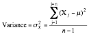
The
standard deviation is the square root of the variance.
The
mean and the standard deviation are the called the first two moments of any
data distribution. A normal distribution can be entirely described by just
these two moments; in other words, the mean and the standard deviation of a
normal distribution suffice to characterize it completely. If a distribution is
not symmetric, the skewness is the third moment that
describes both the direction and the magnitude of the asymmetry and the
kurtosis (the fourth moment) measures the fatness of the tails
of the distribution relative to a normal distribution.