Dealing with Distress in Valuation

CHAPTER 1

INTRODUCTION TO VALUATION

Discounted cash flow and relative valuations are designed to value healthy firms and fall short when used to value firms where there is a substantial probability that the firms may not be in existence in 6 months, a year or two years, because of their inability to make debt payments or cover operating expenses. The degree to which traditional valuation models misvalue distressed firms will vary, depending upon the care with which expected cash flows are estimated, the ease with which these firms can access external capital market and the consequences of distress. In this paper, we will begin by looking at the underpinnings of discounted cash flow valuation, why DCF models do not explicitly consider the possibility of distress and when analysts can get away with ignoring distress. We will follow up by considering ways in which we can adjust discounted cashflow models to explicitly allow for the possibility of distress. In the final part of the paper, we consider how distress is considered (or as is more often, ignored) in relative valuation and ways of adjusting multiples for the possibility of failure.

The Underpinnings of Discounted Cash flow Valuation

Consider how we value a firm in a discounted cash flow world. We begin by projecting expected cash flows for a period, we estimate a terminal value at the end of the period that captures what we believe the firm will be worth at that point in time and we then discount the cash flows back at a discount rate that reflects the riskiness of the firm’s cash flows. This approach is an extraordinarily flexible one and can be stretched to value firms ranging from those with predictable earnings and little growth to those in high growth with negative earnings and cash flows.

Implicit in this approach, though, is the assumption that a firm is a going concern, with potentially an infinite life. The terminal value is usually estimated by assuming that earnings grow at a constant rate forever (a perpetual growth rate). Even when the terminal value is estimated using a multiple of revenues or earnings, this multiple is derived by looking at publicly traded firms (usually healthy ones).

The Possibility and Consequences of Financial Distress

Growth is not inevitable and firms may not remain as going concerns. In fact, even casual empirical observation suggests that a very large number of firms, especially smaller and higher growth firms, will not survive and will go out of business. Some will fail because they borrow money to fund their operations and then are unable to make these debt payments. Other will fail because they do not have the cash to cover their operating needs.

But what are the consequences of financial failure? Firms that are unable to make their debt payments have to liquidate their assets, often at bargain basement prices, and use the cash to pay off debt. If there is any cash left over, which is highly unlikely, it will be paid out to equity investors. Firms that are unable to make their operating payments also have to offer themselves to the highest bidder, and the proceeds will be distributed to the equity investors.

Distress in Discounted Cash flow Valuation

Given the likelihood and consequences of distress, it seems foolhardy to assume that we can ignore this possibility when valuing a firm, and particularly so, when we are valuing firms in poor health and with substantial debt obligations. So, what you might wonder, are the arguments offered by proponents of discounted cash flow valuation for not explicitly considering the possibility of firms failing? We will consider five reasons often provided by for this oversight. The first two reasons are offered by analysts who believe that there is no need to consider distress explicitly, and the last three reasons by those who believe that discounted cashflow valuations already incorporate the effect of distress.

1. We value only large, publicly traded firms and distress is very unlikely for these firms.

It is true that the likelihood of distress is lower for larger, more established firms, but experience suggests that even these firms can become distressed. The last few months of 2001 saw the astonishing demise of Enron, a firm that had a market capitalization in excess of $ 70 billion just a few months previously At the end of 2001, analysts were openly discussing the possibility that large firms like Kmart and Lucent Technologies would be unable to make their debt payments and may have to declare bankruptcy.

The other problem with this argument, even if you accept the premise, is that smaller, high growth firms are traded and need to be valued just as much as larger firms. In fact, you could argue that the need for valuation is greater for smaller firms, where the uncertainty and the possibility of pricing errors are greater.

2. We assume that access to capital is unconstrained

In valuation, as in much of corporate finance, we assume that a firm with good investments has access to capital markets and can raise the funds it needs to meet its financing and investment needs. Thus, firms with great growth potential will never be forced out of business because they will be able to raise capital (more likely equity than debt) to keep going.

In buoyant and developed financial markets, this assumption is not outlandish. Consider, for instance, the ease with which new economy companies with negative earnings and few if any assets were able to raise new equity in the late 1990s. However, even in a market as open and accessible as the United States, access to capital dried up as investors drew back in 2000 and 2001. In summary, then, you may have been able to get away with the assumption that firms with valuable assets will not be forced into a distress sale in 1998 and 1999, but that assumption would have been untenable in 2001.

3. We adjust the discount rate for the possibility of distress

The discount rate is the vehicle we use to adjust for risk in discounted cash flow valuation. Riskier firms have higher costs of equity, higher costs of debt and usually have higher costs of capital than safer firms. A reasonable extension of this argument would be that a firm with a greater possibility of distress should have a higher cost of capital and thus a lower firm value.

The argument has merit up to a point. The cost of capital for a distressed firm, estimated correctly, should be higher than the cost of capital for a safer firm. If the distress is caused by high financial leverage, the cost of equity should be much higher. Since the cost of debt is based upon current borrowing rates, it should also climb as the firm becomes more exposed to the risk of bankruptcy and the effect will be exacerbated if the tax advantage of borrowing also dissipates (as a result of operating losses).

Ultimately though, the adjustment to value that results from using a higher discount rate is only a partial one. The firm is still assumed to generate cash flows in perpetuity, though the present value is lower. A significant portion of the firm’s current value still comes from the terminal value. In other words, the biggest risk of distress that is the loss of all future cash flows is not adequately captured in value.

4. We adjust the expected cash flows for the possibility of distress

To better understand this adjustment, it is worth reviewing what the expected cash flows in a discounted cash flow valuation are supposed to measure. The expected cash flow in a year should be the probability-weighted estimate of the cash flows under all scenarios for the firm, ranging from the best to the worst case. In other words, if there is a 30% chance that a firm will not survive the next year, the expected cash flow should reflect both this probability and the resulting cash flow. In practice, we tend to be far sloppier in our estimation of expected cash flows. In fact, it is not uncommon to use an exogenous estimate of the expected growth rate (from analyst estimates) on the current year’s earnings or revenues to generate future values. Alternatively, we often map out an optimistic path to profitability for unprofitable firms and use this path as the basis for estimating expected cash flows.

We could estimate the expected cash flows under all scenarios and use the expected values in our valuation. Thus, the expected cash flows would be much lower for a firm with a significant probability of distress. Note, though, that contrary to conventional wisdom, this is not a risk adjustment. We are doing what we should have been doing in the first place and estimating the expected cash flows correctly. If we wanted to risk-adjust the cash flows, we would have to adjust the expected cash flows even further downwards using a certainty equivalent.[1] If we do this, though, the discount rate used would have to be the riskfree rate and not the risk-adjusted cost of capital.

As a practical matter, it is very difficult to adjust expected cash flows for the possibility of distress. Not only do we need to estimate the probability of distress each year, we have to keep track of the cumulative probability of distress as well. This is because a firm that becomes distressed in year 3 loses its cash flows not just in that year but in all subsequent years.

5. 5.We assume that even in distress, the firm will be able to receive as proceeds the present value of expected cash flows from its assets

The problem with distress, from a DCF standpoint, is not that the firm ceases to exist but that all cash flows beyond that point in time are lost. Thus, a firm with great products and potentially a huge market may never see this promise converted into cash flows because it goes bankrupt early in its life. If we assume that this firm can sell itself to the highest bidder for a distress sale value that is equal to the present value of expected future cash flows, however, distress does not have to be considered explicitly.

This is a daunting assumption because we are not only assuming that a firm in distress has the bargaining power to demand fair market value for its assets, but we are also assuming that it can do this not only with assets in place (investments it has already made and products that it has produced) but with growth assets (products that it may have been able to produce in the future).

Recapping…

In summary, the failure to explicitly consider distress in discounted cash flow valuation will not have a material impact in value if any the following conditions hold:

1. There is no possibility of bankruptcy, either because of the firm’s size and standing or because of a government guarantee.

2. Easy and free access to capital markets allows firms with good investments to raise debt or equity capital to sustain themselves through bad times, thus ensuring that these firms will never be forced into a distress sale.

3. You used expected cash flows that incorporate the likelihood of distress and a discount rate that is adjusted for the higher risk associated with distress. In addition, the firm will receive sale proceeds that are equal to the present value of expected future cash flows as a going concern in the event of a distress sale.

Adapting Discounted Cash flow Valuation to Distress Situations

When will the failure to consider distress in discounted cash flow valuation have a material impact on value? If the likelihood of distress is high, access to capital is constrained (by internal or external factors) and distress sale proceeds are significantly lower than going concern values, discounted cash flow valuations will overstate firm and equity value, even if the cash flows and the discount rates are correctly estimated. In this section, we will consider several ways of incorporating the effects of distress into the estimated value.

Simulations

In traditional valuation, we estimate expected values for each of the input variables. For instance, in valuing a firm, we may assume an expected growth rate in revenues of 30% a year and that the expected operating margin will be 10%. In reality, each of these variables has a distribution of values, which we condense into an expected value. Simulations attempt to utilize the information in the entire distribution, rather than just the expected value, to arrive at a value. By looking at the entire distribution, simulations provide us with an opportunity to deal explicitly with distress.

Steps in Simulation

Before you begin running the simulations, you will have to decide the circumstances which will constitute distress and what will happen in the event of distress. For example, you may determine that cumulative operating losses of more than $ 1 billion over three years will push the firm into distress and that it will sell its assets for 25% of book value in that event. The parameters for distress will vary not only across firms, based upon their size and asset characteristics, but also on the state of financial markets and the overall economy. A firm that has three bad years in a row in a healthy economy with rising equity markets may be less exposed to default than a similar firm in the middle of a recession. The steps in the simulation are as follows:

Step 1: The first step involves choosing those variables whose expected values will be replaced by distributions. While there may be uncertainty associated with every variable in valuation, only the most critical variables might be chosen at this stage. For instance, revenue growth and operating margins may be the key variables that you choose to build distributions for.

Step 2: You choose a probability distribution for each of the variables. There are a number of choices here, ranging from discrete probability distributions (probabilities are assigned to specific outcomes) to continuous distributions (the normal or exponential distribution). In making this choice, the following factors should be considered:

· the range of feasible outcomes for the variable; (e.g., the revenues cannot be less than zero, ruling out any distribution that requires the variable to take on large negative values, such as the normal distribution).

· the experience of the company on this variable. Data on a variable, such as operating margins historically, may help us determine the type of distribution that best describes it.

While no distribution will provide a perfect fit, the distribution that best fits the data should be used.

Step 3: Next, the parameters of the distribution chosen for each variable are estimated. The number of parameters will vary from distribution to distribution; for instance, the mean and the variance have to be estimated for the normal distribution, while the uniform distribution requires estimates of the minimum and maximum values for the variable.

Step 4: One outcome is drawn from each distribution; the variable is assumed to take on that value for that particular simulation. To make the analysis richer, you can repeat this process each year and allow for correlation across variables and across time.[2]

Step 5: The expected cash flows are estimated based upon the outcomes drawn in step 4. If the firm meets the criteria for a going concern, defined before the simulation, you will then discount the cash flows to arrive at a conventional estimate of discounted cash flow value. If it fails to meet the criteria, you will value it as a distressed firm.

Step 6: Steps 4 and 5 are repeated until a sufficient number of simulations have been conducted. In general, the more complex the distribution (in terms of the number of values the variable can take on and the number of parameters needed to define the distribution) and the greater the number of variables, the larger this number will be.

Step 7: Each simulation will generate a value, going concern or distressed as the case may be, for the firm. The average across all simulated values will be the value of the firm. You should also be able to assess the probability of default from the simulation and the effect of distress on value.

Limitations

The primary limitation of simulation analysis is the information that is required for it to work. In practice, it is difficult to choose both the right distribution to describe a variable and the parameters of that distribution. When these choices are made carelessly or randomly, the output from the simulation may look impressive but actually conveys no valuable information.

Modified Discounted Cash flow Valuation

You can adapt discounted cash flow valuation to reflect some or most of the effects of distress on value. To do this, you will to bring in the effects of distress into both expected cash flows and discount rates.

Estimating Expected Cash flows

To consider the effects of distress into a discounted cash flow valuation, you have to incorporate the probability that your firm will not survive into the expected cash flows. In its most complete form, this would require that you consider all possible scenarios, ranging from the most optimistic to the most pessimistic, assign probabilities to each scenario and cash flows under each scenario, and estimate the expected cash flows each year.

where p_jt is the probability of scenario j in period t and Cashflow_jt is the cashflow under that scenario and in that period. These inputs have to be estimated each year, since the probabilities and the cash flows are likely to change from year to year.

A short-cut, albeit an approximate one, would require estimates for only two scenarios – the going concern scenario and the distress scenario. For the going concern scenario, you could use the expected growth rates and cash flows estimated under the assumption that the firm will be nursed back to health. Under the distress scenario, you would assume that the firm will be liquidated for its distress sale proceeds. Your expected cash flow for each year then would be:

where p_{Going concern, t} is the cumulative probability that the firm will continue as a going concern through period t. The probabilities of distress will have to be estimated for each year and the cumulative probability of surviving as a going concern can then be written as follows:

where p_{distress, t} is the probability that the firm will become distressed in period t. For example, if a firm has 20% chance of distress in year 1 and a 10% chance of distress in year 2, the cumulative probability of surviving as a going concern over two years can be written as:

Cumulative probability of survival over 2 years = (1- .20) (1 - .10) = .72 or 72%

Estimating Discount Rates

In conventional valuation, we often estimate the cost of equity using a regression beta and the cost of debt by looking at the market interest rates on publicly traded bonds issued by the firm. For firms with a significant probability of distress, these approaches can lead to inconsistent estimates. Consider first the use of regression betas. Since regression betas are based upon past prices over long periods (two to five years, for instance), and distress occurs over shorter periods, you will find that these betas will understate the true risk in the distressed firm.[3] With the interest rates on corporate bonds, you run into a different problem. The yields to maturity on the corporate bonds of firms that are viewed as distressed reach extremely high levels, largely because the interest rates are computed based upon promised cash flows (coupons and face value) rather than expected cash flows. The presumption in a going concern valuation is that the promised cash flows have to be made for the firm to remain a going concern, and it is thus appropriate to base the cost of debt on promised rather than expected cash flows. For a firm with a significant likelihood of distress, this presumption is clearly unfounded.

What are the estimation options for distressed firms? To estimate the cost of equity, you should use the bottom-up unlevered beta (the weighted average of unlevered betas of the businesses that your firm operates in) and the current market debt to equity ratio of the firm. Since distressed firms often have high debt to equity ratios, brought about largely as a consequence of dropping stock prices, this will lead to levered betas that are significantly higher than regression betas[4]. If you couple this with the reality that most distressed firms are in no position to get any tax advantages from debt, the levered beta will become even higher.

Levered beta = Bottom-up Unlevered beta (1 + (1- tax rate) (Debt to Equity ratio))

Note, though, that it is reasonable to re-estimate debt to equity ratios and tax rates for future years based upon your expectations for the firm and adjust the beta to reflect these changes. To estimate the cost of debt for a distressed firm, we would recommend using the interest rate based upon the firm’s bond rating. While this will still yield a high cost of debt, it will be more reasonable than the yield to maturity when default is viewed as imminent.[5]

Finally, to compute the cost of capital, you need to estimate the weights on debt on equity. In the initial year, you should use the current market debt to capital ratio (which may be very high for a distressed firm). As your make your forecasts for future years and build in your expectations of improvements in profitability, you should adjust your debt ratio towards more reasonable levels. The conventional practice of using target debt ratios for the entire valuation period (which reflect industry averages or the optimal mix) can lead to misleading estimates of value for firms that are significantly over levered.

Limitations of Approach

The biggest roadblock to using this approach is that even in its limited form, it is difficult to estimate the cumulative probabilities of distress (and survival) each year for the forecast period. Consequently, the expected cash flows may not incorporate the effects of distress completely. In addition, it is difficult to bring both the going concern and the distressed firm assumptions into the same model. We attempt to do so using probabilities, but the two approaches make different and sometimes contradictory assumptions about how markets operate and how distressed firms evolve over time.

Dealing with Distress Separately

An alternative to the modified discounted cash flow model presented in the last section is to separate the going concern assumptions and the value that emerges from it from the effects of distress. To value the effects of distress, you estimate the cumulative probability that your firm will become distressed over your forecast period, and the proceeds that you estimate you will get from the distress sale. The value of the firm can then be written as:

Firm Value = Going concern value * (1-p_Distress )+ Distress sale value * p_Distress

where p_distress is the cumulative probability of distress over the valuation period. In addition to making valuation simpler, it also allows us to make consistent assumptions within each valuation.

You may wonder about the differences between this approach and the far more conventional one of estimating liquidation value for deeply distressed firms. You can consider the distress sale value to be a version of liquidation value, and if you assume that the probability of distress is one, the firm value will, in fact, converge on liquidation value. The advantage of this approach is that it allows us to consider the possibility that even distressed firms have a chance (albeit small) of becoming going concerns.

Going Concern DCF

To value a firm as a going concern, you consider only those scenarios where the firm survives. The expected cash flow is estimated only across these scenarios and thus should be higher than the expected cash flow estimated in the modified discounted cash flow model. When estimating discount rates, we make the assumption that debt ratios will, in fact, decrease over time, if the firm is over levered, and that the firm will derive tax benefits from debt as it turns the corner on profitability. This is consistent with the assumption that the firm will remain a going concern. Most discounted cash flow valuations that we observe in practice are going concern valuations, though they may not come with the tag attached.

Estimating the Probability of Distress

A key input to this approach is the estimate of the cumulative probability of distress over the valuation period. In this section, we will consider three ways in which we can estimate this probability. The first is a statistical approach (a probit) where we relate the probability of distress to a firm’s observable characteristics – firm size, leverage and profitability, for instance – by contrasting firms that have gone bankrupt in prior years with firms that did not. The second is a less data intensive approach, where we use the bond rating for a firm, and the empirical default rates of firms in that rating class to estimate the probability of distress. The third is to use the prices of corporate bonds issued by the firm to back out the probability of distress.

a. Statistical Approaches

The fact that hundreds of firms go bankrupt every year provides us with a rich database that can be examined to evaluate both why bankruptcy occurs and how to predict the likelihood of future bankruptcy. One of the earliest studies that used this approach was by Altman (1968), where he used linear discriminant analysis to arrive at a measure that he called the Z score. In this first paper, that he has since updated several times, the Z score was a function of five ratios:

Z = 0.012 (Working capital/ Total Assets) + 0.014 (Retained Earnings/ Total Assets) + 0.033 (EBIT/ Total Assets) + 0.006 (Market value of equity/ Book value of total liabilities) + 0.999 (Sales/ Total Assets)

Altman argued that you could compute the Z scores for firms and use them to forecast which firms would go bankrupt, and he provided evidence to back up his claim. Since his study, both academics and practitioners have developed their own versions of these credit scores.

Notwithstanding its usefulness in predicting bankruptcy, linear discriminant analysis does not provide a probability of bankruptcy. To arrive at such an estimate, we use a close variant – a probit. In a probit, we begin with the same data that was used in linear discriminant analysis, a sample of firms that survived a specific period and firms that did not. We develop an indicator variable, that takes on a value of zero or one, as follows:

Distress Dummy = 0 for any firm that survived the period

= 1 for any firm that went bankrupt during the period

We then consider information that would have been available at the beginning of the period that may have allowed us to separate the firms that went bankrupt from the firms that did not. For instance, we could look at the debt to capital ratios, cash balances and operating margins of all of the firms in the sample at the start of the period – you would expect firms with high debt to capital ratios, low cash balances and negative margins to be more likely to go bankrupt. Finally, using the dummy variable as our dependent variable and the financial ratios (debt to capital and operating margin) as independent variables, we look for a relationship:

Distress Dummy = a + b (Debt to Capital) + c (Cash Balance/ Value) + d (Operating Margin)

If the relationship is statistically and economically significant, we have the basis for estimating probabilities of bankruptcy.[6]

One advantage of this approach is that it can be extended to cover the likelihood of distress at firms without significant debt. For instance, you could relate the likelihood of distress at young, technology firms to the cash-burn ratio, which measures how much cash a firm has relative to its operating cash needs.[7]

b. Based upon Bond Rating

Many firms, especially in the United States, have bonds that are rated for default risk by the ratings agencies. These bond ratings not only convey information about default risk (or at least the ratings agency’s perception of default risk) but come with a rich history. Since bonds have been rated for decades, we can look at the default experience of bonds in each ratings class. Assuming that the ratings agencies have not significantly altered their ratings standards, we can use these default probabilities as inputs into discounted cash flow valuation models. Altman (2001) has estimated the cumulative probabilities of default for bonds in different ratings classes over five and ten-year periods and the estimates are reproduced in the table below:

Table: Bond Rating and Probability of Default – 1971 - 2001

Rating	Cumulative Probability of Distress
	5 years	10 years
AAA	0.03%	0.03%
AA	0.18%	0.25%
A+	0.19%	0.40%
A	0.20%	0.56%
A-	1.35%	2.42%
BBB	2.50%	4.27%
BB	9.27%	16.89%
B+	16.15%	24.82%
B	24.04%	32.75%
B-	31.10%	42.12%
CCC	39.15%	51.38%
CC	48.22%	60.40%
C+	59.36%	69.41%
C	69.65%	77.44%
C-	80.00%	87.16%

As elaboration, the cumulative default probability for a BB rated bond over ten years is 16.89%.[8]

What are the limitations of this approach? The first is that we are delegating the responsibility of estimating default probabilities to the ratings agencies and we assume that they do it well. The second is that we are assuming that the ratings standards do not shift over time. The third is that the table measures the likelihood of default on a bond, but it does not indicate whether the defaulting firm goes out of business. Many firms continue to operate as going concerns after default.

We can illustrate the use of this approach with Global Crossing. At the end of 2001, Global Crossing had been assigned a bond rating of CCC by Standard and Poors. Based upon this bond rating and the history of defaults between 1971 and 2001, we would have estimated a cumulative probability of bankruptcy of 51.38% over 10 years for the firm.

c. Based upon Bond Price

The conventional approach to valuing bonds discounts promised cash flows back at a cost of debt that incorporates a default spread to come up with a price. Consider an alternative approach. You could discount the expected cash flows on the bond, which would be lower than the promised cash flows because of the possibility of default, at the riskfree rate to price the bond. If we assume that a constant annual probability of default, we can write the bond price as follows for a bond with fixed coupon maturing in N years.

Bond Price =

This equation can now be used, in conjunction with the price on a traded corporate bond to back out the probability of default.

While this approach has the attraction of being a simple one, we would hasten to add the following caveats in using it. First, note that you not only need to find a straight bond issued by the company – special features such as convertibility will render the approach unusable – but the bond price has to be available. If the corporate bond issue is privately placed, this will not be feasible. Second, the probabilities that are estimated may be different for different bonds issued by the same firm. Some of these differences can be traced to the assumption we have made that the annual probability of default remains constant and others can be traced to the mis-pricing of bonds. Finally, as with the previous approach, failure to make debt payments does not always result in the cessation of operations.

Illustration 1: Estimating the probability of bankruptcy using bond price: Global Crossing

Global Crossing has a 12% coupon bond with 8 years to maturity trading at $ 653. To estimate the probability of default (with a treasury bond rate of 5% used as the riskfree rate):

653 =

Solving for the probability of bankruptcy[9], we get

p_Distress = Annual probability of default = 13.53%

To estimate the cumulative probability of distress over 10 years:

Cumulative probability of surviving 10 years = (1 - .1353)¹⁰ = 23.37%

Cumulative probability of distress over 10 years = 1 - .2337 = .7663 or 76.63%

Estimating Distress Sale Proceeds

Once you have estimated the probability that your firm will be unable to make its debt payments and will cease to exist, you have to consider the logical follow-up question. What happens then? As noted earlier in the paper, it is not distress per se that is the problem but the fact that firms in distress have to sell their assets for less than the present value of the expected future cash flows from existing assets and expected future investments. Often, they may be unable to claim even the present value of the cash flows generated even by existing investments. Consequently, a key input that we need to estimate is the expected proceeds in the event of a distress sale. We have three choices:

a. Estimate the present value of the expected cash flows in a discounted cash flow model, and assume that the distress sale will generate only a percentage (less than 100%) of this value. Thus, if the discounted cash flow valuation yields $ 5 billion as the value of the assets, you may assume that the value will only be $ 3 billion in the event of a distress sale.

b. Estimate the present value of expected cash flows only from existing investments as the distress sale value. Essentially, you are assuming that a buyer will not pay for future investments in a distress sale. In practical terms, you would estimate the distress sale value by considering the cash flows from assets in place as a perpetuity (with no growth).

c. The most practical way of estimating distress sale proceeds is to consider the proceeds as a percent of book value of assets, based upon the experience of other distressed firms. Thus, the fact that distressed telecomm companies are able to sell their assets for 20% of book value would indicate that the distress sale proceeds would be 20% of the book value of the assets of your firm.

Note that many of the issues that come up when estimating distress sale proceeds – the need to sell at below fair value, the urgency of the need to sell – are issues that are relevant when estimating liquidation value.

Illustration 2: Estimating Distress Sale Proceeds in January 2002: Global Crossing

To estimate the expected proceeds in the event of a distress sale, we considered several factors. First, the sluggish growth in the economy clearly does not bode well for any firm trying to sell its assets in a liquidation. Second, the fact that a large number of telecomm firms are in distress and looking for potential buyers is also likely to weigh down the proceeds in a sale. In fact, PSInet, another telecomm firm that had recently been forced into a distress sale, was able to receive less than 10% of its book value in the sale. For Global Crossing, we will assume that the distress sale proceeds will be 15% of the book value of the non-cash assets.

Book value of non-cash assets = $14,531 million

Distress sale value = 15% of book value = .15*14531 = $ 2,180 million

Since the firm has debt outstanding (in face value terms) of $7,647 million, the equity investors will receive nothing in the event of a distress sale, even if we consider the cash and marketable securities of $2,260 million that the firm has on its books.

Illustration 3: Valuing Global Crossing with Distress valued separately

To value Global Crossing with distress valued separately, we will begin with a going concern valuation of Global Crossing and then consider the distress sale proceeds:

1. Valuing Global Crossing as a going concern

Global Crossing provides managed data and voice products over a fiber optic network. Over its three-year history, the firm has increased revenues from $420 million in 1998 to $4,040 million in 2001, but it has gone from an operating income of $120 million in 1998 to an operating loss of $1,895 million in 2001[10]. In addition, the firm is capital intensive and reported substantial capital expenditures ($4,289 million) and depreciation ($1,436 million) in 2000.

In making the valuation, we assume that there will be no revenue growth in the first year (to reflect a slowing economy) and that revenue growth will be brisk for the following 4 years and then taper off to a stable growth rate of 5% in the terminal phase, that EBITDA as a percent of sales will move from the current level (of about –10%) to a industry average of 30%. by the end of the tenth year and that capital expenditures will be ratcheted down over the next two years to maintenance levels. Table 1 summarizes our assumptions on revenue growth, EBITDA/Sales and reinvestment needs over the next 10 years.

Table 1: Assumptions for Valuation

	Revenue	EBITDA/ Revenues	Growth rate in Capital Spending	Growth rate in Depreciation	Working capital as % of Revenue
1		-3%	-20%	10%	3.00%
2	40.00%		-50%	10%	3.00%
3	30.00%	5.00%	-30%	10%	3.00%
4	20.00%	10.00%	5%	10%	3.00%
5	10.00%	15.00%	5%	-50%	3.00%
6	10.00%	18.00%	5%	-30%	3.00%
7	10.00%	21.00%	5%	5%	3.00%
8	8.00%	24.00%	5%	5%	3.00%
9	6.00%	27.00%	5%	5%	3.00%
10	5.00%	30.00%	5%	5%	3.00%

For both revenue growth and improvement in EBITDA margins, we assume that the larger changes occur in the earlier years. Note that the changes in depreciation lag the changes in capital spending – the capital spending is cut first and depreciation drops later. Finally, we assume that the firm will need to set aside 3% of the revenue change each year into working capital based upon the industry averages.

With these forecasts, we estimated revenues, operating income and after-tax operating income each year for the high growth period in Table 2. To estimate taxes, we consider the net operating losses carried forward into 2001 of $2,075 million and add on the additional losses that we expect in the first few years of the projection.

Table 2: Expected after-tax operating income to firm: Global Crossing

Year	Revenues	EBITDA	Depreciation	EBIT	NOL at beginning of year	Taxes	EBIT (1-t)
1	$3,804	-$95	$1,580	-$1,675	$2,075	0	-$1,675
2	$5,326	$0	$1,738	-$1,738	$3,750	$0	-$1,738
3	$6,923	$346	$1,911	-$1,565	$5,487	$0	-$1,565
4	$8,308	$831	$2,102	-$1,272	$7,052	$0	-$1,272
5	$9,139	$1,371	$1,051	$320	$8,324	$0	$320
6	$10,053	$1,809	$736	$1,074	$8,004	$0	$1,074
7	$11,058	$2,322	$773	$1,550	$6,931	$0	$1,550
8	$11,942	$2,508	$811	$1,697	$5,381	$0	$1,697
9	$12,659	$3,038	$852	$2,186	$3,685	$0	$2,186
10	$13,292	$3,589	$894	$2,694	$1,498	$419	$2,276
Terminal	$13,957	$4,187	$939	$3,248	$0	$1,137	$2,111

The accumulated losses over the first nine years shield the firm from paying taxes until the tenth year. After that point, we assume a marginal tax rate of 35%.[11]

Finally, we estimated free cash flows to the firm with our assumptions about capital expenditures and working capital.

Table 3: Expected free cashflows to the firm: Global Crossing

Year	EBIT (1-t)	Capital Expenditures	Depreciation	Change in working capital	FCFF
1	-$1,675	$3,431	$1,580	$0	-$3,526
2	-$1,738	$1,716	$1,738	$46	-$1,761
3	-$1,565	$1,201	$1,911	$48	-$903
4	-$1,272	$1,261	$2,102	$42	-$472
5	$320	$1,324	$1,051	$25	$22
6	$1,074	$1,390	$736	$27	$392
7	$1,550	$1,460	$773	$30	$832
8	$1,697	$1,533	$811	$27	$949
9	$2,186	$1,609	$852	$21	$1,407
10	$2,276	$1,690	$894	$19	$1,461
Terminal	$2,111	$2,353	$939	$20	$677

The firm uses debt liberally to fund these investments and had book value of debt outstanding of $7,647 million at the end of 2001. We estimated a market value for the debt of $4,923 million.[12] Based upon its market capitalization (for equity) of $1,649 million at the time of this valuation, we estimated a market debt to capital ratio for the firm.

Debt to capital

Equity to capital

To estimate the bottom-up beta, we begin with an unlevered beta of 0.7527 (based upon all publicly traded telecomm services firms) and estimate the levered beta for the firm:

Levered beta = Unlevered beta ( 1 + (1- tax rate) (Debt/Equity))

= 0.7527 (1 + (1-0) (4923/1649)) = 3.00

Using a bottom-up beta of 3.00 for the equity and a cost of debt of 12.80% based upon the current rating for the firm, we can estimate a cost of capital for the next 5 years. (The riskfree rate is 4.8% and the risk premium is 4%.)

Cost of equity = 4.8% + 3 (4%) = 17.40%

After-tax cost of debt = 12.8% (1-0) = 12.8% (The firm does not pay taxes)

Cost of capital = 16.80% (0.2509) + 12.8% (0.7491) = 13.80%

In stable growth, after year 10, we assume that the beta will decrease to 1.00 and that the pre-tax cost of debt will decrease to 8%. The adjustment occurs in linear increments from years 6 through 10 as shown in Table 4

Table 4: Cost of capital – Global Crossing

Year	1-5	6	7	8	9	10	Terminal
Tax Rate		0%	0%	0%	0%	16%	35%
Beta	3.00	2.60	2.20	1.80	1.40	1.00	1.00
Cost of Equity	16.80%	15.20%	13.60%	12.00%	10.40%	8.80%	8.80%
Cost of Debt	12.80%	11.84%	10.88%	9.92%	8.96%	6.76%	5.20%
Debt Ratio	74.91%	67.93%	60.95%	53.96%	46.98%	40.00%	40.00%
Cost of Capital	13.80%	12.92%	11.94%	10.88%	9.72%	7.98%	7.36%

To estimate the reinvestment rate in the terminal year, we assume that Global Crossing would earn its cost of capital of 7.36% in perpetuity after year 10, and that the expected growth rate would be 5%. This yields a reinvestment rate of 67.93%.

Reinvestment rate in stable growth

Expected FCFF in terminal year

Terminal value

Discounting the operating cashflows and the terminal value back to the present, we arrive at an estimate of the value of the operating assets of $5,530 million. Note, though, that almost of this value comes from our presumption that Global Crossing will not only survive but become profitable, which is the source of the large terminal value. Adding back the cash and marketable securities held by the firm ($2,260 million) and subtracting out the value of debt ($4,923 million) and the estimated value of management options outstanding ($14.3 million)[13], we arrive at a value of equity of $2.852 billion. Dividing by the number of shares outstanding results in a value per share of $3.22.

Value of the operating assets of the firm = $5,529.92

+ Cash and Marketable Securities = $2,260.00

Market Value of Debt = $4,922.75

Market Value of Equity = $2,867.17

Value of Options Outstanding (See option worksheet) = $14.31

Value of Equity in Common Stock = $2,852.86

Value of Equity per Share = $3.22

Valued as a going concern, you would assign a value of $3.22 per share to Global Crossing’s equity.

Dealing with Distress

In illustration 1 we estimated the cumulative probability of distress for Global Crossing to be 76.63% over the next 10 years, and in illustration 2, we estimated the distress sale proceeds to be 15% of book value, based upon how much the assets of other bankruptcy telecomm firms were receiving in the market place currently. Combining these two inputs, we arrive at an estimate of an expected value for the operating assets with distress built into the assumptions:

Expected Value of Operating Assets = 5530 (1 - .7663) + 2180 (.2337) = $2,962.90 million

If we add back the cash and marketable securities and net out the debt, we arrive at an adjusted value of equity for the firm.

Value of the firm = $2,962.90

+ Cash and Marketable Securities = $2,260.00

Market Value of Debt = $4,922.75

Market Value of Equity = $2,031.98

Value of Options Outstanding (See option worksheet) = $14.31

Value of Equity in Common Stock = $2,017.67

Value of Equity per Share = $0.02

One limitation of this approach is that it does not consider the fact that equity has limited liability. In other words, if distress occurs and the value of the operating assets is less than the debt outstanding (as is inevitable), equity investors will get nothing from their investment but will not be required to make up the difference. We can estimate a more realistic value of equity by taking a weighted average of equity per share:

Value of equity = $3.22 (1- .7663) + $ 0.00 (.7663) = $0.75

One way to read this difference is to consider the first estimate of value ($0.02) as the value without limited liability and the second estimate ($0.75) as the value to equity investors of limited liability.

Adjusted Present Value (APV)

In the adjusted present value (APV) approach, we begin with the value of the firm without debt. As we add debt to the firm, we consider the net effect on value by considering both the benefits and the costs of borrowing. To do this, we assume that the primary benefit of borrowing is a tax benefit and that the most significant cost of borrowing is the added risk of bankruptcy.

Steps in APV

We estimate the value of the firm in three steps. We begin by estimating the value of the firm with no leverage. We then consider the present value of the interest tax savings generated by borrowing a given amount of money. Finally, we evaluate the effect of borrowing the amount on the probability that the firm will go bankrupt, and the expected cost of bankruptcy. It is in this last element that we can consider the possibility of distress and its consequences for value.

The first step in this approach is the estimation of the value of the unlevered firm. This can be accomplished by valuing the firm as if it had no debt, i.e., by discounting the expected free cash flow to the firm at the unlevered cost of equity. In the special case where cash flows grow at a constant rate in perpetuity, the value of the firm is easily computed.

Value of Unlevered Firm =

where FCFF₀ is the current after-tax operating cash flow to the firm, r_u is the unlevered cost of equity and g is the expected growth rate. In the more general case, you can value the firm using any set of growth assumptions you believe are reasonable for the firm.

The inputs needed for this valuation are the expected cash flows, growth rates and the unlevered cost of equity. To estimate the latter, we can compute the unlevered beta of the firm.

where

bunlevered = Unlevered beta of the firm

bcurrent = Current equity beta of the firm

t = Tax rate for the firm

D/E = Current debt/equity ratio

This unlevered beta can then be used to arrive at the unlevered cost of equity.

The second step in this approach is the calculation of the expected tax benefit from a given level of debt. This tax benefit is a function of the tax rate of the firm and is discounted at the cost of debt to reflect the riskiness of this cash flow. If the tax savings are viewed as a perpetuity,

Value of Tax Benefits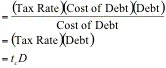

The tax rate used here is the firm’s marginal tax rate and it is assumed to stay constant over time. If we anticipate the tax rate changing over time, we can still compute the present value of tax benefits over time, but we cannot use the perpetual growth equation cited above.

The third step is to evaluate the effect of the given level of debt on the default risk of the firm and on expected bankruptcy costs. In theory, at least, this requires the estimation of the probability of default with the additional debt and the direct and indirect cost of bankruptcy. If p_a is the probability of default after the additional debt and BC is the present value of the bankruptcy cost, the present value of expected bankruptcy cost can be estimated.

PV of Expected Bankruptcy cost

You can use the approaches described in the last section to arrive at an estimate of the probability of bankruptcy. You can also consider the difference between the value of a firm as a going concern and the distress sale value as the cost of bankruptcy. Thus, if the present value of expected cash flows is $ 5 billion – the going concern value – and the distress sale proceeds is expected to be only 25% of the book value of $ 4 billion, the bankruptcy cost is $ 4 billion.

Expected bankruptcy cost = $ 5 billion - .25 (4 billion) = $ 4 billion

Limitations

The adjusted present value approach is best suited for firms that are distressed because they have too much debt. It cannot be used for firms that face the possibility of distress because they have insufficient cash to meet their operating obligations. The estimation challenges abound. In particular, attaching a value to expected bankruptcy cost can be problematic.

Illustration 4: Valuing Global Crossing: Adjusted Present Value

To value Global Crossing on an adjusted present value basis, we would first need to value the firm as an unlevered entity. We can do this by using the unlevered cost of equity as the cost of capital.

Unlevered beta for Global Crossing[14] = 0.7527

Using the riskfree rate of 4.8% and the market risk premium of 4%,

Unlevered cost of equity for Global Crossing = 4.8% + 0.7527 (4%) = 7.81%

We use this cost of equity as the cost of capital and discount the expected free cashflows to the firm shown earlier in table 3. (Note that the terminal value is left unchanged. We will continue to assume that the firm will earn its cost of capital on investments after year 10)

Table 5: Present Value of FCFF at Unlevered Cost of Equity

Year	FCFF	Terminal Value	PV at 7.81%
1	-$3,526		-$3,270.85
2	-$1,761		-$1,515.31
3	-$903		-$720.38
4	-$472		-$349.17
5	$22		$15.02
6	$392		$249.55
7	$832		$491.64
8	$949		$519.81
9	$1,407		$715.26
10	$1,461	$28,683	$14,210.82

The unlevered firm value is $14,211 million. To this we should add the expected tax benefits of debt. Since the firm is losing money and has substantial net operating losses, the expected tax benefits accrue almost entirely after year 10. Consequently, we assume no significant tax benefits[15]. To estimate the bankruptcy cost, we consider the difference between the going concern value of $14,211 million and the distress sale proceeds estimate of $2,180 million (estimated in illustration 2) as the bankruptcy cost. Multiplying this by the probability of bankruptcy estimated in illustration 1 yields the expected cost of bankruptcy:

Adjusted Present Value of Global Crossing’s assets = Unlevered firm value + Present value of tax benefits – Expected bankruptcy costs = 14,211 + 0 – 0.7663 ( 14,211 – 2,180) = $4,992 million

Adding back the cash and marketable securities and subtracting out debt yields a value of equity for Global Crossing:

APV of Global Crossing Assets = $ 4, 992 million

+ Cash & Marketable Securities = $ 2,260 million

- Market value of Debt = $ 4,923 million

Value of Equity = $2,259 million

Value per share = $2,259 million/ 886.47 = $2.55

Relative Valuation

Most valuations, including those of distressed firms, are relative valuations. In particular, firms are valued using multiples and groups of comparable firms. An open question then becomes whether the effects of distress are reflected in relative valuations and, if not, how best to do so.

Distress in Relative Valuation

It is not clear how distress is incorporated into an estimate of relative value. Consider how relative valuation is most often done. You choose a group of firms that you believe are comparable to your firm. Usually, you pick firms in the same business that your firm is in as your comparable firms. You then standardize prices by computing a multiple – price earnings, price to book, enterprise value to sales or enterprise value to EBITDA. Finally, you examine how your firm measures up on this multiple, relative to the comparable firms. While this time honored approach is used for distressed firms as well, the issues listed below generally are unique to distressed firms:

1. Revenue and EBITDA multiples are used more often to value distressed firms than healthy firms. The reasons are pragmatic. Multiple such as price earnings or price to book value often cannot even be computed for a distressed firm. Analysts therefore move up the income statement looking for a positive number. For firms that make heavy infrastructue investments, where depreciation and amortization is a significant charge against operating income and there are substantial interest expenses, the EBITDA is often positive while net income is negative. For some firms, even EBITDA is negative and revenue multiples are only multiples that yield positive values.

2. Analysts who are aware of the possibility of distress often consider them subjectively when they compare the multiple for the firm they are analyzing to the industry average. For example, assume that the average telecomm firm trades at 2 times revenues and that the firm you are analyzing trades at 1.25 times revenues. Assume also that the firm that you are analyzing has substantially higher default risk than the average telecomm firm. You may conclude that the firm is not undervalued even though it trades at a significant discount on the average, because of the potential for default. The perils of subjective adjustment are obvious. Barring the most egregious misvaluations, analysts will find a way to justify their prior biases about firms.

Adapting Relative Valuation to Distress

Is there a way in which relative valuation can be adapted to cover distressed firms? We believe so, though the adjustments tend to be much more approximate than those described in the discounted cash flow section.

Choosing the Comparables

To value a distressed firm, you can find a group of distressed firms in the same business and look at how much the market is willing to pay for them. For instance, you

could value a troubled telecomm firm by looking at the enterprise value to sales (or book capital) multiples at which other troubled telecomm firms trade. While there is promise in this approach, it works only if a large number of firms in a sector slip into financial trouble at the same time. In addition, by categorizing firms as distressed or not distressed firms, you run the risk of lumping together firms that are distressed to different degrees.

One possible way to expand this approach is to look at distressed firms across the whole market, rather than just the sector in which your firm operates. This will allow for a larger sample though there is the possible disadvantage that a troubled grocery store may be in a better position (in terms of generating distress sale proceeds) than a troubled technology company.

Illustration 5: Choosing comparables

To value Global Crossing, we considered only telecomm service firm with negative operating income and high leverage (market debt to capital ratios that exceed 75%). We measured book capital as the sum of the book values of equity and debt at the end of the most recent financial year. Our objective was to arrive at a sample of telecomm firms that have a significant likelihood of distress. Table 6 summarizes the enterprise value/ book capital ratios for these firms:

Table 6: Distressed Telecomm Firms

Company Name	Value to Book Capital	EBIT	Market Debt to Capital Ratio
SAVVIS Communications Corp	0.80	-83.67	75.20%
Talk America Holdings Inc	0.74	-38.39	76.56%
Choice One Comm. Inc	0.92	-154.36	76.58%
FiberNet Telecom Group Inc	1.10	-19.32	77.74%
Level 3 Communic.	0.78	-761.01	78.89%
Global Light Telecom.	0.98	-32.21	79.84%
Korea Thrunet Co. Ltd Cl A	1.06	-114.28	80.15%
Williams Communications Grp	0.98	-264.23	80.18%
RCN Corp.	1.09	-332.00	88.72%
GT Group Telecom Inc Cl B	0.59	-79.11	88.83%
Metromedia Fiber 'A'	0.59	-150.13	91.30%
Global Crossing Ltd.	0.50	-15.16	92.75%
Focal Communications Corp	0.98	-11.12	94.12%
Adelphia Business Solutions	1.05	-108.56	95.74%
Allied Riser Communications	0.42	-127.01	95.85%
CoreComm Ltd	0.94	-134.07	96.04%
Bell Canada Intl	0.84	-51.69	96.42%
Globix Corp.	1.06	-59.35	96.94%
United Pan Europe Communicatio	1.01	-240.61	97.27%
Average	0.87

Global Crossing trades at 50% of book capital invested, significantly lower than the average ratio across these distressed firms. We could view this as indicative of the fact that Global Crossing is under valued on a relative basis, though that conclusion would be justified only if we assume that the firms are exposed to equal degrees to financial distress.

Adjusting the Multiple

A second possibility is to look for objective ways of adjusting the multiple for distress. Consider one possible solution. You could examine the multiple of revenues or operating income at which firms in different ratings classes trade at to get a measure of the discount (if any) that is being applied by the market for the degree of distress to which a firm is exposed. If there are enough firms in the sector that you are analyzing in each ratings class, you could do this on a sector basis. If there are not, you could look at the multiple across the entire market and examine differences across bond rating classes.

Illustration 6: Adjusted Multiple: Global Crossing

Looking at all telecomm firms, and categorizing them based upon bond ratings, we were able to estimate the value to book ratios by bond rating class:

Bond Rating Value to Book Capital Ratio

A 1.70

BBB 1.61

BB 1.18

B 1.06

CCC 0.88

CC 0.61

The differences between ratings classes provide us with an indication of the discount that you would apply when valuing distressed firms. For instance, Global Crossing with its CCC ratings should have a multiple that is roughly half that of a healthy A rated firm in the same sector.

Considering the Possibility of Distress Explicitly

One of the adaptations that we suggested for discounted cash flow valuation was an explicit assessment of default risk and a firm value that was a weighted estimate of a going concern value and a distress sale value. For a distressed firm in a sector where the average firm is healthy, this approach offers promise. You can estimate the value of the distressed firm using the comparable firms and consider it the going concern value. For instance, if healthy firms in the business trade at 2 times revenues, you would multiple your firm’s revenues by 2 to arrive at the going concern value. You could then estimate the firm value as follows:

Firm Value = Going concern relative value * (1-p_Distress )+ Distress sale value * p_Distress

The probability of distress and the distress sale value would be estimated just as they were in the last section. This approach makes the most sense when valuing a firm that is distressed in a sector containing mostly healthy firms, since the prior two approaches could not be used here.

In some cases, you may have to use forecasted values for revenues and operating income to arrive at the going concern value, especially if current revenues and operating income are adversely impacted by the overhang of distress.

Illustration 7: Forward Multiples and Distress

Consider the forecasts of revenues and EBITDA made in table 2 for Global Crossing. While the firm is losing a substantial amount of money currently, we are forecasting a return to financial health. In year 5, for instance, Global Crossing is expected to have an EBITDA of $1,371 million on revenues of $9,139 million. Using the average enterprise value/EBITDA multiple of 7.2 at which healthy telecomm firms[16] trade, we can estimate an expected enterprise value in year 5.

Expected Enterprise value in year 5 = EBITDA₅ * EV/ EBITDA_{Current for healthy telecomm firms}

= 1,371 * 7.2 = $9,871 million

You can estimate the present value of this estimated value by discounting back at Global Crossing’s cost of capital.

Enterprise value today = 9871/1.138⁵ = $5,172 million

This, of course, is based upon the assumption that Global Crossing will become a healthy firm. Using the probability of survival (23.37%) and distress (76.63%) estimated earlier, we can value Global Crossing’s operating assets today:

Estimated Enterprise Value

= Going Concern Value (p_{Going Concern}) + Distres Sale Value (1 - p_{Going Concern})

= 5172 (.2337) + 2180 (.7663) = $2,879 million

Note that the estimate of the distress sale value of $2,180 million was made earlier in illustration 2. Adding back the cash balance of the firm ($ 2,260 million) and subtracting out debt ($4923 million) yields a value for the equity:

Enterprise Value = $ 2,879 million

+ Cash & Marketable Securities = $ 2,260 million

- Debt = $4,923 million

Value of Equity = $216 million

Value per share = $216/ 886.47 =$ 0.24

From Firm to Equity Value in Distressed Firms

In conventional valuation, you subtract the market value of the debt from firm value to arrive at equity value. When valuing distressed firms, you have to consider two specific issues. The first is the shifting debt load at these firms, since these firms are often in the process of restructuring and renegotiating debt, can make identifying the dollar debt due sat a point in time a hazardous exercise. The second is that equity in distressed firms often take on option characteristics and may need to be analyzed as options.

The Shifting Debt Load

In addition to having a substantial amount of debt, distressed firms often have very complicated debt structures. Not only do they owe money to a number of different creditors, but the debt itself often is usually complex – convertible, callable and filled with special features demanded by the creditors for their own protection. In addition, distressed firms are often in the process of negotiating with debt holders, trying to convince them to change the terms of the debt and, in some cases, convert their debt into equity. Consequently, the value of the debt can change dramatically from day to day, thus affecting the value of equity, even if the enterprise value does not.

When estimating the value of debt in a distressed firm, you should consider doing the following:

• · Rather than relying on the last available financial statements for the available debt, you should try to obtain an updated estimate of the outstanding debt. This may be difficult to do when the debt negotiations are private (between the distressed firm and the lenders.
• · You should update the estimated market value of debt frequently, since the default risk of distressed firms can change substantially from period to period. Even if the debt is not traded, it is never appropriate with distressed firms to use the book value of equity as a proxy for the market value of debt. Instead, you should estimate the market value of debt, treating book debt like a corporate bond.
• · When confronted with convertible debt, you should strip the conversion option from the debt and treat it as equity. Again, a simple way to do this is to value the convertible debt as if it were straight debt – this will yield the debt portion of the convertible debt – and consider the difference between the market value of the convertible debt and the straight debt portion as equity.

Equity as an Option

In distressed firms with a substantial debt obligation, equity takes on the characteristics of an option. In particular, if the value of the firm’s assets is less than the face value of the outstanding debt, as is often the case with a distressed firm, you can argue that equity investors have the option to liquidate the firm if the asset value climbs above the face value of the debt but cannot lose more than their equity investment, if asset value drops below:

Condition Equity investor’s payoff on liquidation

If Value of assets > Face value of debt: Asset value – Face Value of debt

Value of assets < Face value of debt: 0

So what are the implications for valuation? To the extent that equity investors value equity as an option, you can argue that the equity in a deeply distressed firm should be the greater of two values – the conventional value of equity, obtained by subtracting the market value of debt from firm value and the value of equity as an option – with the liquidation value of the assets representing the value of the underlying asset and the face value of debt the strike price. This approach to valuing equity in deeply distressed firms is described more fully in Damodaran (2001).[17]

Conclusion

Every asset, financial as well as real, has a value. The key to successfully investing in and managing these assets lies in understanding not only what the value is but also the sources of the value. Any asset can be valued, but some assets are easier to value than others and the details of valuation will vary from case to case. Thus, the valuation of a share of a real estate property will require different information and follow a different format than the valuation of a publicly traded stock. What is surprising, however, is not the differences in valuation techniques across assets, but the degree of similarity in basic principles. There is undeniably uncertainty associated with valuation. Often that uncertainty comes from the asset being valued, though the valuation model may add to that uncertainty.

This chapter lays out a philosophical basis for valuation, together with a discussion of how valuation is or can be used in a variety of frameworks, from portfolio management to corporate finance.

A philosophical basis for valuation

It was Oscar Wilde who described a cynic as one who “knows the price of everything, but the value of nothing”. He could very well have been describing some equity research analysts and many investors, a surprising number of whom subscribe to the 'bigger fool' theory of investing, which argues that the value of an asset is irrelevant as long as there is a 'bigger fool' willing to buy the asset from them. While this may provide a basis for some profits, it is a dangerous game to play, since there is no guarantee that such an investor will still be around when the time to sell comes.

A postulate of sound investing is that an investor does not pay more for an asset than its worth. This statement may seem logical and obvious, but it is forgotten and rediscovered at some time in every generation and in every market. There are those who are disingenuous enough to argue that value is in the eyes of the beholder, and that any price can be justified if there are other investors willing to pay that price. That is patently absurd. Perceptions may be all that matter when the asset is a painting or a sculpture, but investors do not (and should not) buy most assets for aesthetic or emotional reasons; financial assets are acquired for the cashflows expected on them. Consequently, perceptions of value have to be backed up by reality, which implies that the price paid for any asset should reflect the cashflows that it is expected to generate. The models of valuation described in this book attempt to relate value to the level and expected growth in these cashflows.

There are many areas in valuation where there is room for disagreement, including how to estimate true value and how long it will take for prices to adjust to true value. But there is one point on which there can be no disagreement. Asset prices cannot be justified by merely using the argument that there will be other investors around willing to pay a higher price in the future.

Generalities about Valuation

Like all analytical disciplines, valuation has developed its own set of myths over time. This section examines and debunks some of these myths.

Myth 1: Since valuation models are quantitative, valuation is objective

Valuation is neither the science that some of its proponents make it out to be nor the objective search for the true value that idealists would like it to become. The models that we use in valuation may be quantitative, but the inputs leave plenty of room for subjective judgments. Thus, the final value that we obtain from these models is colored by the bias that we bring into the process. In fact, in many valuations, the price gets set first and the valuation follows.

The obvious solution is to eliminate all bias before starting on a valuation, but this is easier said than done. Given the exposure we have to external information, analyses and opinions about a firm, it is unlikely that we embark on most valuations without some bias. There are two ways of reducing the bias in the process. The first is to avoid taking strong public positions on the value of a firm before the valuation is complete. In far too many cases, the decision on whether a firm is under or over valued precedes the actual valuation[18], leading to seriously biased analyses. The second is to minimize the stake we have in whether the firm is under or over valued, prior to the valuation.

Institutional concerns also play a role in determining the extent of bias in valuation. For instance, it is an acknowledged fact that equity research analysts are more likely to issue buy rather than sell recommendations,[19] i.e., that they are more likely to find firms to be undervalued than overvalued. This can be traced partly to the difficulties they face in obtaining access and collecting information on firms that they have issued sell recommendations and to the pressure that they face from portfolio managers, some of whom might have large positions in the stock. In recent years, this trend has been exacerbated by the pressure on equity research analysts to deliver investment banking business.

When using a valuation done by a third party, the biases of the analyst(s) doing the valuation should be considered before decisions are made on its basis. For instance, a self-valuation done by a target firm in a takeover is likely to be positively biased. While this does not make the valuation worthless, it suggests that the analysis should be viewed with skepticism.

The Biases in Equity Research

The lines between equity research and salesmanship blur most in periods that are characterized by “irrational exuberance”. In the late 1990s, the extraordinary surge of market values in the companies that comprised the new economy saw a large number of equity research analysts, especially on the sell side, step out of their roles as analysts and become cheerleaders for these stocks. While these analysts might have been well meaning in their recommendations, the fact that the investment banks that they worked for were leading the charge on new initial public offerings from these firms exposed them to charges of bias and worse.

In 2001, the crash in the market values of new economy stocks and the anguished cries of investors who had lost wealth in the crash created a firestorm of controversy. There were congressional hearing where legislators demanded to know what analysts knew about the companies they recommended and when they knew it, statements from the SEC about the need for impartiality in equity research and decisions taken by some investment banking to create at least the appearance of objectivity. At the time this book went to press, both Merrill Lynch and CSFB had decided that their equity research analysts could no longer hold stock in companies that they covered. Unfortunately, the real source of bias – the intermingling of investment banking business and investment advice – was left untouched.

Should there be government regulation of equity research? We do not believe that it would be wise, since regulation tends to be heavy handed and creates side costs that seem to quickly exceed the benefits. A much more effective response can be delivered by portfolio managers and investors. The equity research of firms that create the potential for bias should be discounted or, in egregious cases, even ignored.

Myth 2: A well-researched and well-done valuation is timeless

The value obtained from any valuation model is affected by firm-specific as well as market-wide information. As a consequence, the value will change as new information is revealed. Given the constant flow of information into financial markets, a valuation done on a firm ages quickly, and has to be updated to reflect current information. This information may be specific to the firm, affect an entire sector or alter expectations for all firms in the market. The most common example of firm-specific information is an earnings report that contains news not only about a firm’s performance in the most recent time period but, more importantly, about the business model that the firm has adopted. The dramatic drop in value of many new economy stocks from 1999 to 2001 can be traced, at least partially, to the realization that these firms had business models that could deliver customers but not earnings, even in the long term. In some cases, new information can affect the valuations of all firms in a sector. Thus, pharmaceutical companies that were valued highly in early 1992, on the assumption that the high growth from the eighties would continue into the future, were valued much less in early 1993, as the prospects of health reform and price controls dimmed future prospects. With the benefit of hindsight, the valuations of these companies (and the analyst recommendations) made in 1992 can be criticized, but they were reasonable, given the information available at that time. Finally, information about the state of the economy and the level of interest rates affect all valuations in an economy. A weakening in the economy can lead to a reassessment of growth rates across the board, though the effect on earnings are likely to be largest at cyclical firms. Similarly, an increase in interest rates will affect all investments, though to varying degrees.

When analysts change their valuations, they will undoubtedly be asked to justify them. In some cases, the fact that valuations change over time is viewed as a problem. The best response may be the one that Lord Keynes gave when he was criticized for changing his position on a major economic issue: “When the facts change, I change my mind. And what do you do, sir?”

Myth 3.: A good valuation provides a precise estimate of value

Even at the end of the most careful and detailed valuation, there will be uncertainty about the final numbers, colored as they are by the assumptions that we make about the future of the company and the economy. It is unrealistic to expect or demand absolute certainty in valuation, since cash flows and discount rates are estimated with error. This also means that you have to give yourself a reasonable margin for error in making recommendations on the basis of valuations.

The degree of precision in valuations is likely to vary widely across investments. The valuation of a large and mature company, with a long financial history, will usually be much more precise than the valuation of a young company, in a sector that is in turmoil. If this company happens to operate in an emerging market, with additional disagreement about the future of the market thrown into the mix, the uncertainty is magnified. Later in this book, we will argue that the difficulties associated with valuation can be related to where a firm is in the life cycle. Mature firms tend to be easier to value than growth firms, and young start-up companies are more difficult to value than companies with established produces and markets. The problems are not with the valuation models we use, though, but with the difficulties we run into in making estimates for the future.

Many investors and analysts use the uncertainty about the future or the absence of information to justify not doing full-fledged valuations. In reality, though, the payoff to valuation is greatest in these firms.

Myth 4: .The more quantitative a model, the better the valuation

It may seem obvious that making a model more complete and complex should yield better valuations, but it is not necessarily so. As models become more complex, the number of inputs needed to value a firm increases, bringing with it the potential for input errors. These problems are compounded when models become so complex that they become ‘black boxes’ where analysts feed in numbers into one end and valuations emerge from the other. All too often the blame gets attached to the model rather than the analyst when a valuation fails. The refrain becomes “It was not my fault. The model did it.”

There are three points we will emphasize in this book on all valuation. The first is the principle of parsimony, which essentially states that you do not use more inputs than you absolutely need to value an asset. The second is that the there is a trade off between the benefits of building in more detail and the estimation costs (and error) with providing the detail. The third is that the models don’t value companies: you do. In a world where the problem that we often face in valuations is not too little information but too much, separating the information that matters from the information that does not is almost as important as the valuation models and techniques that you use to value a firm.

Myth 5: To make money on valuation, you have to assume that markets are inefficient

Implicit often in the act of valuation is the assumption that markets make mistakes and that we can find these mistakes, often using information that tens of thousands of other investors can access. Thus, the argument, that those who believe that markets are inefficient should spend their time and resources on valuation whereas those who believe that markets are efficient should take the market price as the best estimate of value, seems to be reasonable.

This statement, though, does not reflect the internal contradictions in both positions. Those who believe that markets are efficient may still feel that valuation has something to contribute, especially when they are called upon to value the effect of a change in the way a firm is run or to understand why market prices change over time. Furthermore, it is not clear how markets would become efficient in the first place, if investors did not attempt to find under and over valued stocks and trade on these valuations. In other words, a pre-condition for market efficiency seems to be the existence of millions of investors who believe that markets are not.

On the other hand, those who believe that markets make mistakes and buy or sell stocks on that basis ultimately must believe that markets will correct these mistakes, i.e. become efficient, because that is how they make their money. This is a fairly self-serving definition of inefficiency – markets are inefficient until you take a large position in the stock that you believe to be mispriced but they become efficient after you take the position.

We approach the issue of market efficiency as wary skeptics. On the one hand, we believe that markets make mistakes but, on the other, finding these mistakes requires a combination of skill and luck. This view of markets leads us to the following conclusions. First, if something looks too good to be true – a stock looks obviously under valued or over valued – it is probably not true. Second, when the value from an analysis is significantly different from the market price, we start off with the presumption that the market is correct and we have to convince ourselves that this is not the case before we conclude that something is over or under valued. This higher standard may lead us to be more cautious in following through on valuations. Given the historic difficulty of beating the market, this is not an undesirable outcome.

Myth 6: The product of valuation (i.e., the value) is what matters; The process of valuation is not important.

As valuation models are introduced in this book, there is the risk of focusing exclusively on the outcome, i.e., the value of the company, and whether it is under or over valued, and missing some valuable insights that can be obtained from the process of the valuation. The process can tell us a great deal about the determinants of value and help us answer some fundamental questions -- What is the appropriate price to pay for high growth? What is a brand name worth? How important is it to improve returns on projects? What is the effect of profit margins on value? Since the process is so informative, even those who believe that markets are efficient (and that the market price is therefore the best estimate of value) should be able to find some use for valuation models.

The Role of Valuation

Valuation is useful in a wide range of tasks. The role it plays, however, is different in different arenas. The following section lays out the relevance of valuation in portfolio management, acquisition analysis and corporate finance.

1. Valuation and Portfolio Management

The role that valuation plays in portfolio management is determined in large part by the investment philosophy of the investor. Valuation plays a minimal role in portfolio management for a passive investor, whereas it plays a larger role for an active investor. Even among active investors, the nature and the role of valuation is different for different types of active investment. Market timers use valuation much less than investors who pick stocks, and the focus is on market valuation rather than on firm-specific valuation. Among security selectors, valuation plays a central role in portfolio management for fundamental analysts and a peripheral role for technical analysts.

The following sub-section describes, in broad terms, different investment philosophies and the role played by valuation in each.

1. Fundamental Analysts: The underlying theme in fundamental analysis is that the true value of the firm can be related to its financial characteristics -- its growth prospects, risk profile and cashflows. Any deviation from this true value is a sign that a stock is under or overvalued. It is a long term investment strategy, and the assumptions underlying it are:

(a) the relationship between value and the underlying financial factors can be measured.

(b) the relationship is stable over time.

(c) deviations from the relationship are corrected in a reasonable time period.

Valuation is the central focus in fundamental analysis. Some analysts use discounted cashflow models to value firms, while others use multiples such as the price-earnings and price-book value ratios. Since investors using this approach hold a large number of 'undervalued' stocks in their portfolios, their hope is that, on average, these portfolios will do better than the market.

2. Franchise Buyer: The philosophy of a franchise buyer is best expressed by an investor who has been very successful at it -- Warren Buffett. "We try to stick to businesses we believe we understand," Mr. Buffett writes[20]. "That means they must be relatively simple and stable in character. If a business is complex and subject to constant change, we're not smart enough to predict future cash flows." Franchise buyers concentrate on a few businesses they understand well, and attempt to acquire undervalued firms. Often, as in the case of Mr. Buffett, franchise buyers wield influence on the management of these firms and can change financial and investment policy. As a long term strategy, the underlying assumptions are that :

(a) Investors who understand a business well are in a better position to value it correctly.

(b) These undervalued businesses can be acquired without driving the price above the true value.

Valuation plays a key role in this philosophy, since franchise buyers are attracted to a particular business because they believe it is undervalued. They are also interested in how much additional value they can create by restructuring the business and running it right.

3. Chartists: Chartists believe that prices are driven as much by investor psychology as by any underlying financial variables. The information available from trading -- price movements, trading volume, short sales, etc. -- gives an indication of investor psychology and future price movements. The assumptions here are that prices move in predictable patterns, that there are not enough marginal investors taking advantage of these patterns to eliminate them, and that the average investor in the market is driven more by emotion rather than by rational analysis.

While valuation does not play much of a role in charting, there are ways in which an enterprising chartist can incorporate it into analysis. For instance, valuation can be used to determine support and resistance lines[21] on price charts.

4. Information Traders: Prices move on information about the firm. Information traders attempt to trade in advance of new information or shortly after it is revealed to financial markets, buying on good news and selling on bad. The underlying assumption is that these traders can anticipate information announcements and gauge the market reaction to them better than the average investor in the market.

For an information trader, the focus is on the relationship between information and changes in value, rather than on value, per se. Thus an information trader may buy an 'overvalued' firm if he believes that the next information announcement is going to cause the price to go up, because it contains better than expected news. If there is a relationship between how undervalued or overvalued a company is and how its stock price reacts to new information, then valuation could play a role in investing for an information trader.

5. Market Timers: Market timers note, with some legitimacy, that the payoff to calling turns in markets is much greater than the returns from stock picking. They argue that it is easier to predict market movements than to select stocks and that these predictions can be based upon factors that are observable.

While valuation of individual stocks may not be of any use to a market timer, market timing strategies can use valuation in at least two ways:

(a) The overall market itself can be valued and compared to the current level.

(b) A valuation model can be used to value all stocks, and the results from the cross-section can be used to determine whether the market is over or under valued. For example, as the number of stocks that are overvalued, using the dividend discount model, increases relative to the number that are undervalued, there may be reason to believe that the market is overvalued.

6. Efficient Marketers: Efficient marketers believe that the market price at any point in time represents the best estimate of the true value of the firm, and that any attempt to exploit perceived market efficiencies will cost more than it will make in excess profits. They assume that markets aggregate information quickly and accurately, that marginal investors promptly exploit any inefficiencies and that any inefficiencies in the market are caused by friction, such as transactions costs, and cannot be arbitraged away.

For efficient marketers, valuation is a useful exercise to determine why a stock sells for the price that it does. Since the underlying assumption is that the market price is the best estimate of the true value of the company, the objective becomes determining what assumptions about growth and risk are implied in this market price, rather than on finding under or over valued firms.

2. Valuation in Acquisition Analysis

Valuation should play a central part of acquisition analysis. The bidding firm or individual has to decide on a fair value for the target firm before making a bid, and the target firm has to determine a reasonable value for itself before deciding to accept or reject the offer.

There are also special factors to consider in takeover valuation. First, the effects of synergy on the combined value of the two firms (target plus bidding firm) have to be considered before a decision is made on the bid. Those who suggest that synergy is impossible to value and should not be considered in quantitative terms are wrong. Second, the effects on value, of changing management and restructuring the target firm, will have to be taken into account in deciding on a fair price. This is of particular concern in hostile takeovers.

Finally, there is a significant problem with bias in takeover valuations. Target firms may be over-optimistic in estimating value, especially when the takeover is hostile, and they are trying to convince their stockholders that the offer price is too low. Similarly, if the bidding firm has decided, for strategic reasons, to do an acquisition, there may be strong pressure on the analyst to come up with an estimate of value that backs up the acquisition.

3. Valuation in Corporate Finance

If the objective in corporate finance is the maximization of firm value[22], the relationship among financial decisions, corporate strategy and firm value has to be delineated. In recent years, management consulting firms have started offered companies advice on how to increase value[23]. Their suggestions have often provided the basis for the restructuring of these firms.

The value of a firm can be directly related to decisions that it makes -- on which projects it takes, on how it finances them and on its dividend policy. Understanding this relationship is key to making value-increasing decisions and to sensible financial restructuring.

Conclusion

Valuation plays a key role in many areas of finance -- in corporate finance, mergers and acquisitions and portfolio management. The models presented in this book will provide a range of tools that analysts in each of these areas will find useful, but the cautionary note sounded in this chapter bears repeating. Valuation is not an objective exercise; and any preconceptions and biases that an analyst brings to the process will find its way into the value.




Questions and Short Problems: Chapter 1

1. The value of an investment is

A. the present value of the cash flows on the investment

B. determined by investor perceptions about it

C. determined by demand and supply

D. often a subjective estimate, colored by the bias of the analyst

E. all of the above

2. There are many who claim that value is based upon investor perceptions, and perceptions alone, and that cash flows and earnings do not matter. This argument is flawed because

A. value is determined by earnings and cash flows, and investor perceptions do not matter.

B. perceptions do matter, but they can change. Value must be based upon something more stable.

C. investors are irrational. Therefore, their perceptions should not determine value.

D. value is determined by investor perceptions, but it is also determined by the underlying earnings and cash flows. Perceptions must be based upon reality.

3. You use a valuation model to arrive at a value of $15 for a stock. The market price of the stock is $25. The difference may be explained by

A. a market inefficiency; the market is overvaluing the stock.

B. the use of the wrong valuation model to value the stock.

C. errors in the inputs to the valuation model.

D. none of the above

E. either A, B, or C. Distressed firms, i.e., firms with negative earnings that are exposed to substantial likelihood of failure, present a challenge to analysts valuing them because so much of conventional valuation is built on the presumption that firms are going concerns. In this paper, we have examined how both discounted cash flow and relative valuation deal (sometimes partially and sometimes not at all) with distress. With discounted cash flow valuation, we suggested four ways in which you can incorporate distress into value – simulations that allow for the possibility that a firm will have to be liquidated, modified discounted cash flow models, where the expected cash flows and discount rates are adjusted to reflect the likelihood of default, separate valuations of the firm as a going concern and in distress and adjusted present value models. With relative valuation, you can adjust your multiples for distress or use other distressed firms as your comparable firms.




References

Altman, E.I., 1968, Financial Ratios, Discriminant Analysis and the Prediction of Corporate Bankruptcy, Journal of Finance, v23, pp 589-609.

Altman, E.I., 2002, Bankruptcy, Credit Risk and High Yield Junk Bonds, Blackwell.

Altman, E.I. and V. Kishore, 2000, The Default Experience of U.S. Bonds, Working Paper, Salomon Center, Stern School of Business, New York University.

Altman, E.I, and P. Arman, 2002, Defaults and Returns on High Yield Bonds, Analysis through 2001, Working Paper, Salomon Center, Stern School of Business, New York University.

Damodaran, A., 2002, Investment Valuation (Second Edition), John Wiley & Sons.

Damodaran, A., Estimating Equity Risk Parameters, Working paper, www.stern.nyu.edu/~adamodar/New_Home_Page/papers.html.

---

[1] A certainty equivalent cashflow replaces an uncertain cash flow with an equivalent riskless cashflow. Thus, an expected cashflow of $ 125 million will be replaced by a riskless cashflow of $ 100 million. The more uncertain the cash flow, the greater the downward adjustment.

[2] For example, you may increase the likelihood of the earnings being low if the earnings in previous years were low and the likelihood of negative margins if revenue growth is low.

[3] As an extreme example, consider estimating a beta for Enron at the end of 2001. The beta estimate from Bloomberg, using 2 years of data, was 1.45. Over three-quarters of this period, Enron was viewed (rightly or wrongly) as a healthy firm with positive earnings. It is only in the last part of the regression period that you see the effects of distress on stock prices and the debt to equity ratio of the firm.

[4] For more on bottom-up betas, refer to Damodaran (2000).

[5] The yields to maturity on bonds issued by companies where there is a significant probability of distress will be stratospheric, because they are based upon the promised cash flows on the bond, rather than expected cashflows.

[6] This looks like a multiple regression. In fact, a probit is a more sophisticated version of this regression with constraints built in ensuring that the probabilities do not exceed one or become negative.

[7] Cash Burn Ratio = Cash Balance/ EBITDA. With negative EBITDA, this yields a measure of the time that it will take the firm to burn through its cash balance.

[8] Altman estimates the probability of default only for AAA, AA, A, BBB, BB, B and CCC bonds. We interpolated to get the rest of the table.

[9] With a 10-year bond, it is a process of trial and error to estimate this value. The solver function in excel accomplishes the same in far less time.

[10] While the financial statements for 2000 had not been released, the trailing 12-month numbers were used for most of the inputs in November 2001

[11] The tax rate in year 10 is less than 35% because of the net operating losses carried forward from the previous year.

[12] To estimate the market value, we discounted the face value of debt and the interest payments back at the estimated pre-tax cost of debt of 12.80%.

[13] The Black-Scholes model was used to estimate the value of the options outstanding. In fact, these options had lost a substantial portion of value because of the drop in the stock price.

[14] We used the unlevered beta of telecomm services firms as the unlevered beta for Global Crossing.

[15] This is conservative. There will be tax benefits after year 10. We could estimate these tax benefits and consider them in present value terms.

[16] We considered only firms with positive operating income and low debt to capital ratios (less than 30%) as healthy firms.

[17] See chapter 30 of the second edition of Investment Valuation for more details on valuing equity in a deeply distressed firm as an option.

[18]This is most visible in takeovers, where the decision to acquire a firm often seems to precede the valuation of the firm. It should come as no surprise, therefore, that the analysis almost invariably supports the decision.

[19]In most years, buy recommendations outnumber sell recommendations by a margin of ten to one. In recent years, this trend has become even stronger.

[20]This is extracted from Mr. Buffett's letter to stockholders in Berkshire Hathaway for 1993.

[21]On a chart, the support line usually refers to a lower bound below which prices are unlikely to move and the resistance line refers to the upper bound above which prices are unlikely to venture. While these levels are usually estimated using past prices, the range of values obtained from a valuation model can be used to determine these levels, i.e., the maximum value will become the resistance level and the minimum value will become the support line.

[22]Most corporate financial theory is constructed on this premise.

[23]The motivation for this has been the fear of hostile takeovers. Companies have increasingly turned to 'value consultants' to tell them how to restructure, increase value and avoid being taken over.