I. Framework

II. The Basis of Technical Analysis

III. The Nature of Technical Analysis

• Investors have used price charts and price patterns as tools for predicting future price movements for as long as there have been financial markets.
• The first studies of market efficiency focused on the relationship between price changes over time, to see if in fact such predictions were feasible.
• Evidence can be classified into two classes
  • studies that focus on short-term (intraday, daily and weekly price movements) price behavior and
  • research that examines long-term (annual and five-year returns) price movements.

a. Serial correlation

• Serial correlation measures the correlation between price changes in consecutive time periods
• Measure of how much price change in any period depends upon price change over prior time period.
  • 0: imply that price changes in consecutive time periods are uncorrelated with each other
  • >0: evidence of price momentum in markets
  • <0: Evidence of price reversals
• From viewpoint of investment strategy, serial correlations can be exploited to earn excess returns.
  • A positive serial correlation would be exploited by a strategy of buying after periods with positive returns and selling after periods with negative returns.
  • A negative serial correlation would suggest a strategy of buying after periods with negative returns and selling after periods with positive returns.
• The correlations must be large enough for investors to generate profits to cover transactions costs.

Author	Data	Variables	Time Interval	Correlation
Kendall & Alexander(28	19 indices - UK	price	1 week 2 weeks 4 weeks	0.131 0.134 0.006
Moore (28)	30 companies - US	log prices	1 week	-0.056
Cootner (28)	45 companies US	log prices	1 week	-0.047
Fama (46)	30 companies - US	log prices	1 day 4 days 9 days	0.026 -0.039 -0.053
King (28)	63 companies - US	log prices	1 month	0.018
Niarchos (119)	15 companies - Greece	log prices	1 month	0.036
Praetz (128)	16 indices 20 companies	log prices	1 week 1 week	0.000 -0.118

• Serial correlations in most markets is small. While there may be statistical significance associated with these correlations, it is unlikely that there is enough correlation to generate excess returns.
• The serial correlation in short period returns is also affected by price measurement issues and the market micro-structure characteristics.
  • Non-trading in some of the components of the index can create a carry-over effect from the prior time period, this can result in positive serial correlation in the index returns.
  • The bid-ask spread creates a bias in the opposite direction, if transactions prices are used to compute returns, since prices have a equal chance of ending up at the bid or the ask price. The bounce that this induces in prices will result in negative serial correlations in returns.

Bid-Ask Spread = Square root of (Serial Covariance in returns)

where the serial covariance in returns measures the covariance between return changes in consecutive time periods.

• In a filter rule, an investor buys an investment if the price rises X% from a previous low and holds the investment until the price drops X% from a previous high. The magnitude of the change (X%) that triggers the trades can vary from filter rule to filter rule. with smaller changes resulting in more transactions per period and higher transactions costs.

• This strategy is based upon the assumption that price changes are serially correlated and that there is price momentum, i.e., stocks which have gone up strongly in the past are more likely to keep going up than go down.
• The following table summarizes results from a study on returns, before and after transactions costs, on a trading strategy based upon filter rules ranging from 0.5% to 20%. ( A 0.5% rule implies that a stock is bought when it rises 0.5% from a previous low and sold when it falls 0.5% from a prior high.)

Value of X	Return with strategy	Return with Buy and Hold	# Transactions with strategy	Return after transactions costs
0.5%	11.5%	10.4%	12,514	-103.6%
1.0%	5.5%	10.3%	8,660	-74.9%
2.0%	0..2%	10.3%	4,764	-45.2%
3.0%	-1.7%	10.1%	2,994	-30.5%
4.0%	0.1%	10.1%	2,013	-19.5%
5.0%	-1.9%	10.0%	1,484	-16.6%
6.0%	1.3%	9.7%	1,071	-9.4%
8.0%	1.7%	9.6%	653	-5.0%
10.0%	3.0%	9.6%	435	-1.4%
12.0%	5.3%	9.4%	289	2.3%
10.3%	224	1.4%	16.0%	4.2%

• The only filter rule that beats the returns from the buy and hold strategy is the 0.5% rule, but it does so before transactions costs. This strategy creates 12,514 trades during the period which generate enough transactions costs to wipe out the principal invested by the investor.
• While this test is an dated, it also illustrates a basic problem with strategies that require frequent short term trading. Even though these strategies may earn excess returns prior to transactions costs, adjusting for these costs can wipe out the excess returns.

• A variant on the filter rule is the relative strength measure, which relates recent prices on stocks or other investments to either average prices over a specified period, say over six months, or to the price at the beginning of the period.
• Stocks which score high on the relative strength measure are considered good investments.
• This investment strategy is also based upon the assumption of price momentum.

• A runs test is a non-parametric variation on the serial correlation, and it is based upon a count of the number of runs, i.e., sequences of price increases or decreases, in the price changes. Thus, the following price changes, where U is an increase and D a decrease would result in the following runs:

UUU DD U DDD UU DD U D UU DD U DD UUU DD UU D UU D

There were 18 runs in this price series of 33 periods.

• The actual number of runs in the price series is compared against the number that can be expected in a series of this length, assuming that price changes are random.
  • If the actual number of runs is greater than the expected number, there is evidence of negative correlation in price changes.
  • If it is lower, there is evidence of positive correlation.

• A study of price changes in the Dow 30 stocks, assuming daily, four-day, nine-day and sixteen day return intervals provided the following results -

DIFFERENCING INTERVAL

Daily Four-day Nine-day Sixteen-day

Actual runs 735.1 175.7 74.6 41.6

Expected runs 759.8 175.8 75.3 41.7

• Based upon these results, there is evidence of positive correlation in daily returns but no evidence of deviations from normality for longer return intervals.
• Long strings of positive and negative changes are, by themselves, insufficient evidence that markets are not random, since such behavior is consistent with price changes following a random walk. It is the recurrence of these strings that can be viewed as evidence against randomness in price behavior.

a. The January Effect

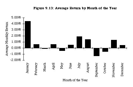
• Studies of returns in the United States and other major financial markets consistently reveal strong differences in return behavior across the months of the year. Figure 9.13 reports average returns by month of the year from 1926 to 1983.

• Returns in January are significantly higher than returns in any other month of the year. This phenomenon is called the year-end or January effect, and it can be traced to the first two weeks in January.
• The January effect is much more accentuated for small firms than for larger firms, and roughly half of the small firm premium, described in the prior section, is earned in the first two days of January. Figure 9.14 graphs returns in January by size and risk class for data from 1935 to 1986.

• A number of explanations have been advanced for the January effect, but few hold up to serious scrutiny.
  • Tax loss selling by investors at the end of the year on stocks which have 'lost money' to capture the capital gain, driving prices down, presumably below true value, in December, and a buying back of the same stocks in January, resulting in the high returns.
  • A second rationale is that the January effect is related to institutional trading behavior around the turn of the years. It has been noted, for instance, that ratio of buys to sells for institutions drops significantly below average in the days before the turn of the year and picks to above average in the months that follow.

b. The Weekend Effect

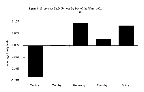
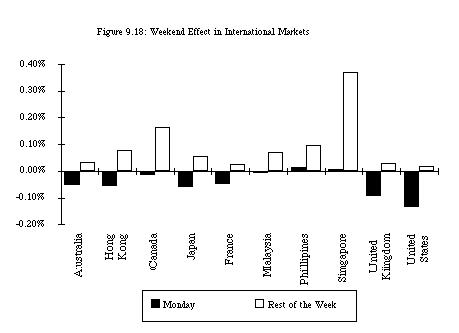
The weekend effect is another phenomenon that has persisted over long periods and over a number of international markets. It refers to the differences in returns between Mondays and other days of the week. Figure 9.17, which graphs returns by days of the week from 1962 to 1978

.

• There are a number of other findings on the Monday effect that have fleshed it out.
  • First, the Monday effect is really a weekend effect since the bulk of the negative returns is manifested in the Friday close to Monday open returns. The returns from intraday returns on Monday are not the culprits in creating the negative returns.
  • Second, the Monday effect is worse for small stocks than for larger stocks.
  • Third, the Monday effect is no worse following three-day weekends than two-day weekends.
• There are some who have argued that the weekend effect is the result of bad news being revealed after the close of trading on Friday and during the weekend. Even if this were a widespread phenomenon, the return behavior would be inconsistent with a rational market, since rational investors would build in the expectation of the bad news over the weekend into the price before the weekend, leading to an elimination of the weekend effect.

• The presence of a strong weekend effect in Japan, which allowed Saturday trading for a portion of the period studies here indicates that there might be a more direct reason for negative returns on Mondays than bad information over the weekend.
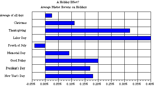
• As a final note, the negative returns on Mondays cannot be just attributed to the absence of trading over the weekend. The returns on days following trading holidays, in general, are characterized by positive, not negative, returns. Figure 9.19 summarizes returns on trading days following major holidays and confirms this pattern.

A summary of the underlying assumptions (Levy)

(1) Market value is determined solely by the interaction of supply and demand

(2) Supply and demand are governed by numerous factors both rational and irrational. The market continually and automatically weighs all these factors. (A random walker would have no qualms about this assumption either. He would however point out that any irrational factors are just as likely to be one side of the market as on the other.)

(3) Disregarding minor fluctuations in the market, stock prices tend to move in trends which persist for an appreciable length of time. ( Random walker would disagree with this statement. For any trend to persist there has to be some collective 'irrationality')

(4) Changes in trend are caused by shifts in demand and supply. These shifts no matter why they occur, can be detected sooner or later in the action of the market itself. (In the financial economist's view the market (through the price) will instantaneously reflect any shifts in the demand and supply. However knowledge that the demand or supply has shifted after it has already been reflected in the price is worthless.)

"It is futile to assign an intrinsic value to a stock certificate. One share of US Steel , for example, was worth $261 in the early fall of 1929, but you could buy it for only $22 in June 1932. By March 1937 it was selling for $126 and just one year later for $38. ... This sort of thing, this wide deivergence between presumed value and intrinsic value, is not the exception; it is the rule; it is going on all the time. The fact is that the real value of US Steel is determined at any give time solely, definitely and inexorably by supply and demand, which are accurately reflected in the transactions consummated on the floor of the exchange.

Of course, the statistics which the fundamentalists study play a part in the supply and demand equation- that is freely admitted. But there are many other factors affecting it. The market price reflects not only the differing fears and guesses and moods, rational and irrational, of hundreds of potential buyers and sellers.. as well as their needs and resources- in total, factors which defy analysis and for which no statistics are obtainable but which nevertheless are all synthesised, weighted and finally expressed in the one precise figure at which a buyer and seller get together and make a deal. This is the only figure that counts.

• Historians who have examined the behavior of financial markets over time have challenged the assumption of rationality that underlies much of efficient market theory.
• They point out to the frequency with speculative bubbles have formed in financial markers, as investors buy into fads or get-rich-quick schemes, and the crashes with these bubbles have ended, and suggest that there is nothing to prevent the recurrence of this phenomenon in today's financial markets. There is some evidence in the literature of irrationality on the part of market players.

• While most experimental studies suggest that traders are rational, there are some examples of irrational behavior in some of these studies.
• One such study was done at the University of Arizona. In an experimental study, traders were told that a payout would be declared after each trading day, determined randomly from four possibilities - zero, eight, 28 or 60 cents. The average payout was 24 cents. Thus the share's expected value on the first trading day of a fifteen day experiment was $3.60 (24*15), the second day was $3.36 .... The traders were allowed to trade each day. The results of 60 such experiments is summarized in the following graph.

• There is clear evidence here of a 'speculative bubble' forming during periods 3 to 5, where prices exceed expected values by a significant amount.
• The bubble ultimately bursts, and prices approach expected value by the end of the period.
• If this is feasible in a simple market, where every investor obtains the same information, it is clearly feasible in real financial markets, where there is much more differential information and much greater uncertainty about expected value.
• Some of the experiments were run with students, and some with Tucson businessmen, with 'real world' experience. The results were similar for both groups.
• Furthermore, when price curbs of 15 cents were introduced, the booms lasted even longer because traders knew that prices would not fall by more than 15 cents in a period. Thus, the notion that price limits can control speculative bubbles seems misguided.

b. Chaos and Non-linear Dynamics in Prices

• The recent use of chaos theory to explain natural phenomena (such as weather patterns) has also generated some interest into its potential uses in explaining stock price behavior.
• Peters, for instance, has tried to model price behavior using the non-linear models that underlie much of chaos theory with mixed results.

• Artificial Intelligence: Software systems that attempt to replicate aspects of human intelligence.
• Expert System: Computerized decision-making technique that embodies knowledge gleaned from experts.
• Neural Network: Tries to mimic human brain processes and learns from mistakes it makes.
• Chaos Theory: Holds that seemingly random event s actually have patterns that computers can detect.

Genetic Algorithm: Problem solving technique useful in identifying and handling anomalies. Evolution is used to find winners.

I. MARKET OVERREACTION: The Contrarian Indicators

Basis: Research in experimental psychology suggests that people tend to overreact to unexpected and dramatic news events. In revising their beliefs, individuals tend to overweight recent information and underweight prior data.

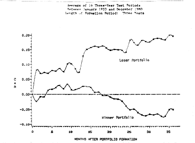
Empirical evidence: If markets overreact then

(1) Extreme movements in stock prices will be followed by subsequent price movements in the opposite direction.

(2) The more extreme the price adjustment, the greater will be the subsequent adjustment

Issues: (1) Why, if this is true, is is that contrarian investors are so few in number or market power that the overreaction to new information is allowed to continue for so long?

(2) In what sense does this phenomenon justify th accusation that the market is inefficient?

(3) Is the market more efficient about incorporating some types of information than others?

Technical trading rules: Contrarian Opinion

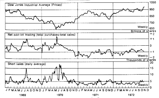
1. Odd-lot trading: The odd-lot rule gives us an indication of what the man on the street thinks about the stock (As he gets more enthusiastic about a stock this ratio will increase).

2. Mutual Fund Cash positions: Historically, the argument goes, mutual fund cash positions have been greatest at the bottom of a bear market and lowest at the peak of a bull market. Hence investing against this statistic may be profitable.

3. Investment Advisory opinion: This is the ratio of advisory services that are bearish. When this ratio reaches the threshold (eg 60%) the contrarian starts buying.

The Shiller Effect: The true value is the present value of all expected future dividends. However the variance in current prices is substantially greater than the variance in this present value.

Technical rules: Breadth of the market

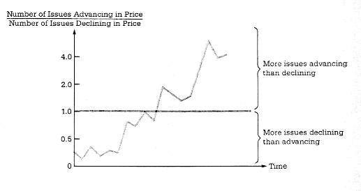
Measure: This is a measure of the number of stocks in the market which have advanced relative to those that have declined. The broader the market, the stronger the demand.

Related measures: (1) Divergence between different market indices (Dow 30 vs NYSE composite) (2) Advance/Decline lines

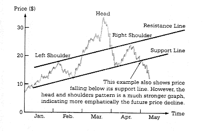
(2) Support and Resistance lines: A common explanation given by technicians for market movements is that markets have support and resistance lines. If either is broken, the market is poised for a major move.

Possible rationale: (1) Institutional buy/sell programs which can be triggered by breakthrough of certain well defined price levels (eg. Dow 1300) (2) Self fulfilling prophecies: How money managers use technical analysts for window dressing.

(3) Moving Averages: A moving average line smooths out fluctuations and enables the chartist to see trends in the stock price. How that trend is interpreted then depends upon the chartist.

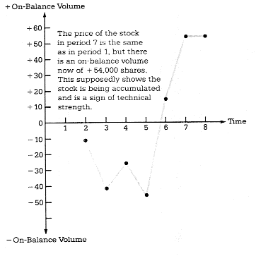
(4) Trading Volume Indicators: Some technical analysts believe that there is information about future price changes in trading volume shifts.

(5) Point and figure charts:

Basis: The argument here is that markets learn slowly. Thus, investors who are a little quicker than the market in assimilating and understanding information will earn excess returns. In addition, if markets learn slowly, there will be price drifts (i.e., prices will move up or down over extended periods) and technical analysis can detect these drifts and take advantage of them.

The Evidence: There is evidence, albeit mild, that prices do drift after significant news announcements. For instance, following up on price changes after large earnings surprises provides the following evidence.

Note the price drift, especially after the most extreme earnings announcements.

Relative Strength rules: The relative strength of a stock is the ratio of its current price to its average over a longer period (eg. six months). The rule suggests buying stocks which have the highest relative strength (which will also be the stocks that have gone up the most in that period).

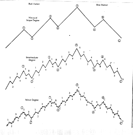
The Elliot Wave: Elliot's theory is that the market moves in waves of various sizes, from those encompassing only individual trades to those lasting centuries, perhaps longer. "By classifying these waves and counting the various classifications it is possible to determine the relative positions of the market at all times". "There can be no bull of bear markets of one, seven or nine waves, for example.

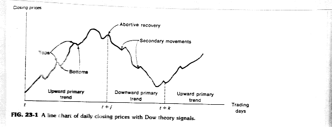
The Dow Theory:" The market is always considered as having three movements, all going at the same time. The first is the narrow movement (daily fluctuations) from day to day. The second is the short swing (secondary movements) running from two weeks to a month and the third is the main movement (primary trends) covering at least four years in its duration.

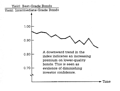
(a) Confidence Index: The confidence index measures the ratio of yields on risky bonds (eg. BBB) to safer bonds (AAA). A higher ratio here is bullish.

(b) Specialists' short sales ratio: Specialists are better informed than the average investor. an increase in their short sales is considered a bearish sign.