Year	Investment	Revenues	EBIT (1-t)	Depreciation	Chg. in WC	FCFF
0	-12500000				-3000000	-15500000
1		30000000	1920000	540000	-150000	2310000
2		31500000	2016000	432000	-157500	2290500
3		33075000	2116800	345600	-165375	2297025
4		34728750	2222640	276480	-173644	2325476
5	-1000000	36465188	2333772	221184	-182326	2372630
6		38288447	2450461	176947	-191442	2435966
7		40202869	2572984	141558	-201014	2513527
8		42213013	2701633	113246	-211065	2603814
9		44323663	2836714	90597	-221618	2705693
10	5500000	46539846	2978550	72478	4653985	13205012

FCFF = EBIT (1-t) + Depreciation + Change in Working Capital

Net Present Value (at cost of capital of 12.5%)= $ 1,067,099 : Accept the Project

Internal Rate of Return = 13.83% > Cost of Capital : Accept the Project

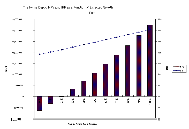
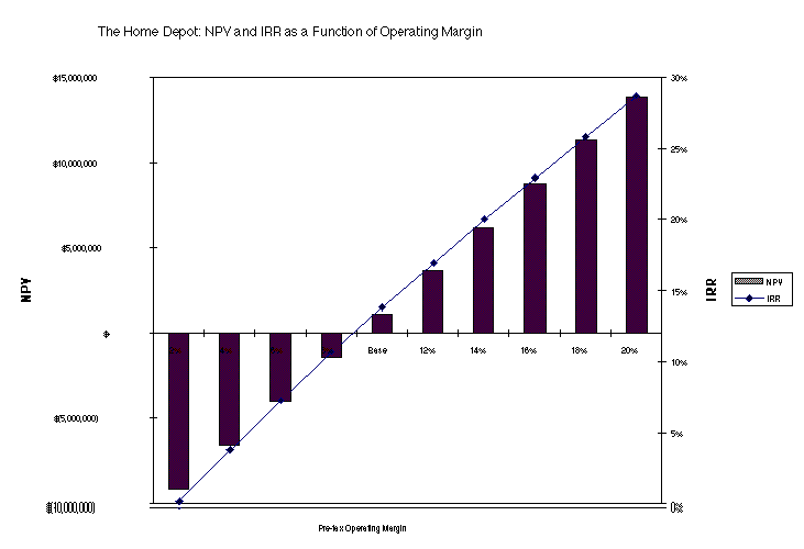
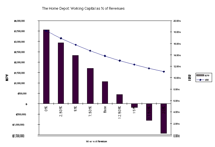
Sensitivity Analysis



A Variant on Sensitivity Analysis: Scenario Analysis

In scenario analysis, specific scenarios are defined, with growth and income characteristics under each. The net present value and internal rates of return for the project are estimated under each scenario ñ



What next?

• Provides a sense of the worst case and best case scenarios, i.e., the potential upside and downside on the project.
• Becomes a factor in analyzing the riskiness of a project; the spread between the net present values becomes a measure of risk.
• Can be used to develop protection. For instance, if a project is very sensitive to shifts in currency rates, currency risk may be hedged away.

* Effects Of Assumptions About Project Lifetime

Consider the following project:

Initial Investment = $1,000,000; Salvage Value after 10 years = $200,000

Initial Working Capital Needs = $100,000; Maintain at 25% of Revenues

Revenues in year 1 = $400,000; Grows at 10% a year;

COGS = 50% of Revenues

Discount rate for project = 15%

Year	Initial Invest.	Revenues	COGS	BTCF	ATCF	WC Chg	NATCF
0	-1100000
1		400000	200000	200000	120000	0	120000
2		440000	220000	220000	132000	10000	122000
3		484000	242000	242000	145200	11000	134200
4		532400	266200	266200	159720	12100	147620
5		585640	292820	292820	175692	13310	162382
6		644204	322102	322102	193261	14641	178620
7		708624	354312	354312	212587	16105	196482
8		779487	389743	389743	233846	17716	216130
9		857436	428718	428718	257231	19487	237743
10		943179	471590	471590	282954	21436	261518

* Monte Carlo Simulations

Step 1: Instead of using an expected value for each of the inputs, develop probability distributions for each of the variables.

Example: In the Home Depot example, assume the following distributions for each of the following variables ñ

Variable Distribution Expected Value Characteristics of the Distribution

1. Revenues General $ 30 million Value Probability

$ 20 million 0.125

$ 25 million 0.1875

$ 30 million 0.375

$ 35 million 0.1875

$ 40 million 0.125

2. Growth Rate Normal 5.00% Standard Deviation = 2.00%

3. Operating Margin Uniform 10.00% Minimum of 2.50%

Maximum of 20.00%

4. WC as % of Rev. Normal 10.00% Standard Deviation = 2.50%

Estimation Issues:

• How do you choose the right probability distribution?

  • Extreme Values for the Variable: For instance, the normal distribution will generally work only for variables that can take on (at least at the limits) values ranging from -_ to +_.
  • Past Experience: The Home Depot, for instance, has opened hundreds of stores and can use the values for the variables from these stores to develop distributions. Thus, the operating margins of the stores can be plotted on a distribution, and a standard distribution can be matched up to it.
• How do you estimate the parameters of the distribution?
  • Past Experience
  • Experiences of competitiors

Step 2: Draw one outcome from each distribution.

Example: In the Home Depot example, assume the following drawings ñ

Variable Drawn Outcome

1. Revenues $ 25 million

2. Growth Rate 6.35%

3. Operating Margin 10.00%

4. WC as % of Rev. 9.16%

Estimation Issues:

• How do you draw an outcome from a distribution?
  • For simpler distributions (uniform, general), a bell jar will work.
  • For more complex distributions, a computer may be necessary (though tables exist)

Step 3: Estimate a net present value, based upon the outcomes drawn

Example: In the Home Depot example, calculate the net present value based upon the outcomes drawn in step 3.
Net Present Value from simulated outcomes = - $13,423
Internal Rate of Return for simulated outcomes = 12.48%

Estimation Issues:

• What if variables are correlated with each other ? (For instance, what if the growth rate is likely to be higher than expected when revenues are higher than expected?)
  • Develop joint distributions for variables that are correlated.

Step 4: Repeat step 2 and 3 a sufficient number of times.

Example: In the Home Depot example, the simulations were repeated 1000 times. The number was set to a fairly large number because

• the distributions were complex
• four variables were changing in the project

Estimation Issues:

• What is a sufficient number?
  • The number of simulations will increase
    • with the complexity of the distribution (more for the exponential, less for the general)
    • with the number of variables that change

Step 5: Compute the summary statistics for the net present values across all the simulations (Expected Value, Standard Deviation, Minimum, Maximum, Percent of time under zero) and plot the net present values on a graph.)

Example: In the Home Depot example, calculate the summary statistics for net present value based upon the simulations.
Net Present Value Internal Rate of Return
Expected Value = $ 1,067,150 Expected Value = 13.84%
Standard Deviation = $ 451,335 Standard Deviation = 0.55%

Coeff. of Variation = $ 451,335/1,067,150 CV of IRR = 0.55%/13.84%

Minimum = -$ 9,504,201 Minimum = -1.21%

Maximum = $ 31,013,450 Maximum = 47.95%
% of time below zero = 20.16% % of time below Discount rate= 20.16%


Step 6: Use the distribution of net present values, rather than just the base case net present value to make your decision.

Example: In the Home Depot example, there are a number of questions that can be answered with this simulation, including

• What is the likelihood that this will be a bad project? (20.16%)
• What is the worst case and best case scenarios? ( Minimum and Maximum values)
• What is the riskiness of this project relative to other projects? (Standard Deviation, CV)

* Decision Trees

Stage 1: At t=0, conduct a $500,000 study of market potential.

Stage 2: If it appears that there is a significant market (assumed to have probability 0.8) at t=1, spend $1,000,000 to build a small plant to manufacture prototypes for use in industry.

Stage 3: If the reaction to the prototypes is good, at t=2, build a larger plant for $10,000,000. The project is expected to generate cash flows for four years, before the patent expires.

Assume that the discount rate is 11.5%.

Time Periods



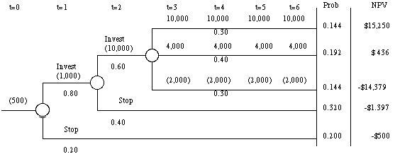
NPV = 0.144* 15,250 + 0.192 * 436 + 0.144 * (14,379) + 0.32 * 1397 + 0.2* (500)

= - $ 338

Note on calculations:

Probability of best case scenario = 0.8 * 0.6 * 0.4 = 0.144

NPV under best case scenario = - 500 - 1000/1.115 - 10,000/1.1152 + 10,000/1.1153 + 10,000/1.1154 + 10,000/1.1155 + 10,000/1.1156 = $15,250

The Abandonment Option

In the example above, assume that you can abandon the project at the end of t=3, if the cashflows turn out to be negative (-2,000).



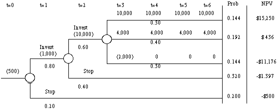
NPV = 0.144* 15,250 + 0.192 * 436 + 0.144 * (11,176) + 0.32 * 1397 + 0.2* (500)

= $124